This function simulates future incidence based on past incidence data, a selection of plausible reproduction numbers (R), and the distribution of the serial interval (time from primary onset to secondary onset).
project(
  x,
  R,
  si,
  n_sim = 100,
  n_days = 7,
  R_fix_within = FALSE,
  model = c("poisson", "negbin"),
  size = 0.03,
  time_change = NULL
)
Arguments
| x | An |
|---|---|
| R | A vector of numbers representing plausible reproduction numbers; for instance, these can be samples from a posterior distribution using the `earlyR` or `EpiEstim` packages. If `time_change` is provided, then it must be a `vector` (for fixed values of R per time window) or a `list` of vectors (for separate distributions of R per time window), with one element more than the number of dates in `time_change`. |
| si | A function computing the serial interval, or a `numeric` vector
providing its mass function, starting a day 1, so that si[i] is the PMF for
serial interval of `i`. The model implicitly assumes that `si[0] = 0`. For
functions, we strongly recommend using the RECON package |
| n_sim | The number of epicurves to simulate. Defaults to 100. |
| n_days | The number of days to run simulations for. Defaults to 14. |
| R_fix_within | A logical indicating if R should be fixed within
simulations (but still varying across simulations). If |
| model | Distribution to be used for projections. Must be one of "poisson" or "negbin" (negative binomial process). Defaults to poisson |
| size | size parameter of negative binomial distribition. Ignored if model is poisson |
| time_change | an optional vector of times at which the simulations should use a different sample of reproduction numbers, provided in days into the simulation (so that day '1' is the first day after the input `incidence` object); if provided, `n` dates in `time_change` will produce `n+1` time windows, in which case `R` should be a list of vectors of `n+1` `R` values, one per each time window. |
Details
The decision to fix R values within simulations
(R_fix_within) reflects two alternative views of the uncertainty
associated with R. When drawing R values at random from the provided
sample, (R_fix_within set to FALSE), it is assumed that R
varies naturally, and can be treated as a random variable with a given
distribution. When fixing values within simulations (R_fix_within
set to TRUE), R is treated as a fixed parameter, and the uncertainty
is merely a consequence of the estimation of R. In other words, the first
view is rather Bayesian, while the second is more frequentist.
Examples
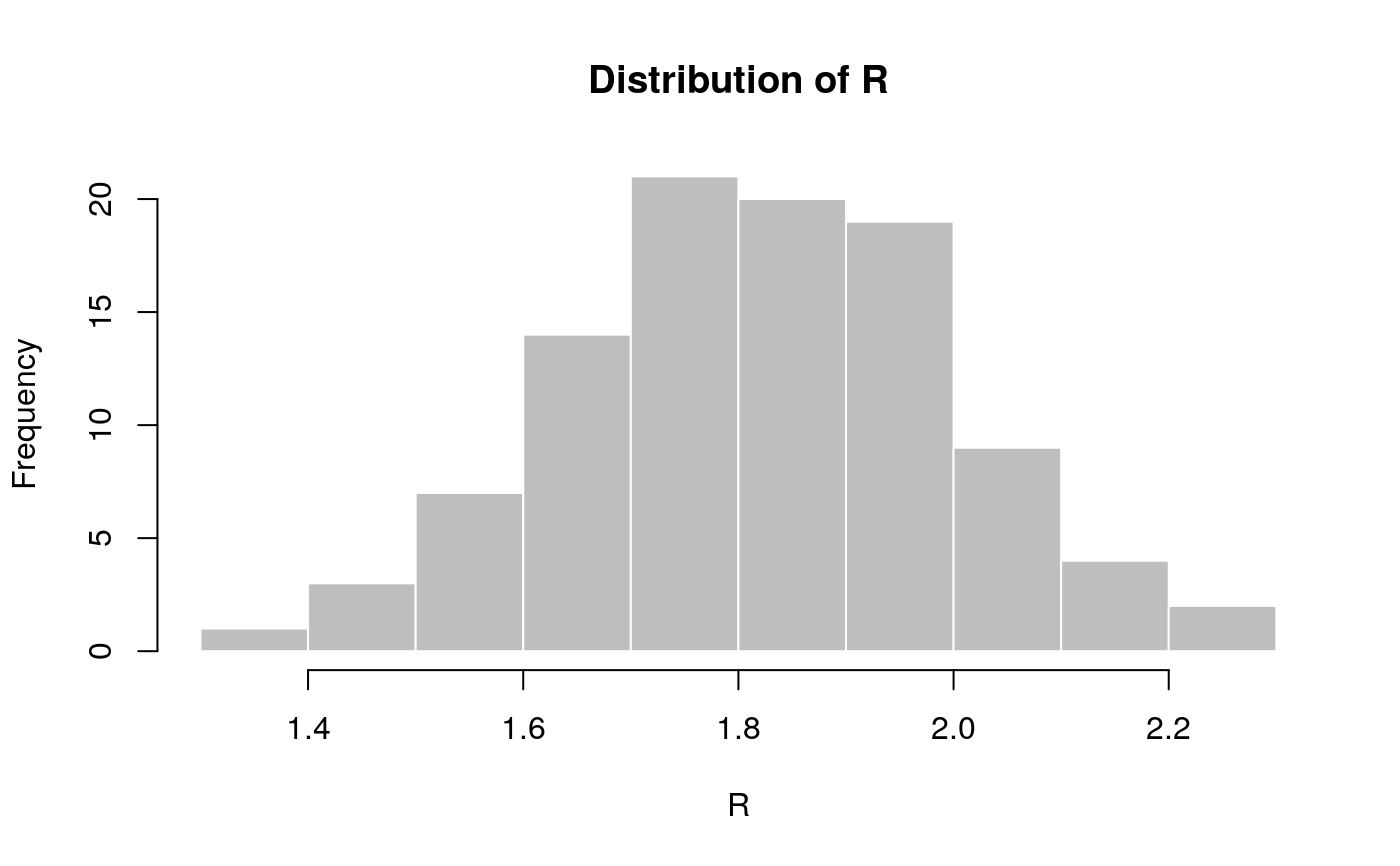
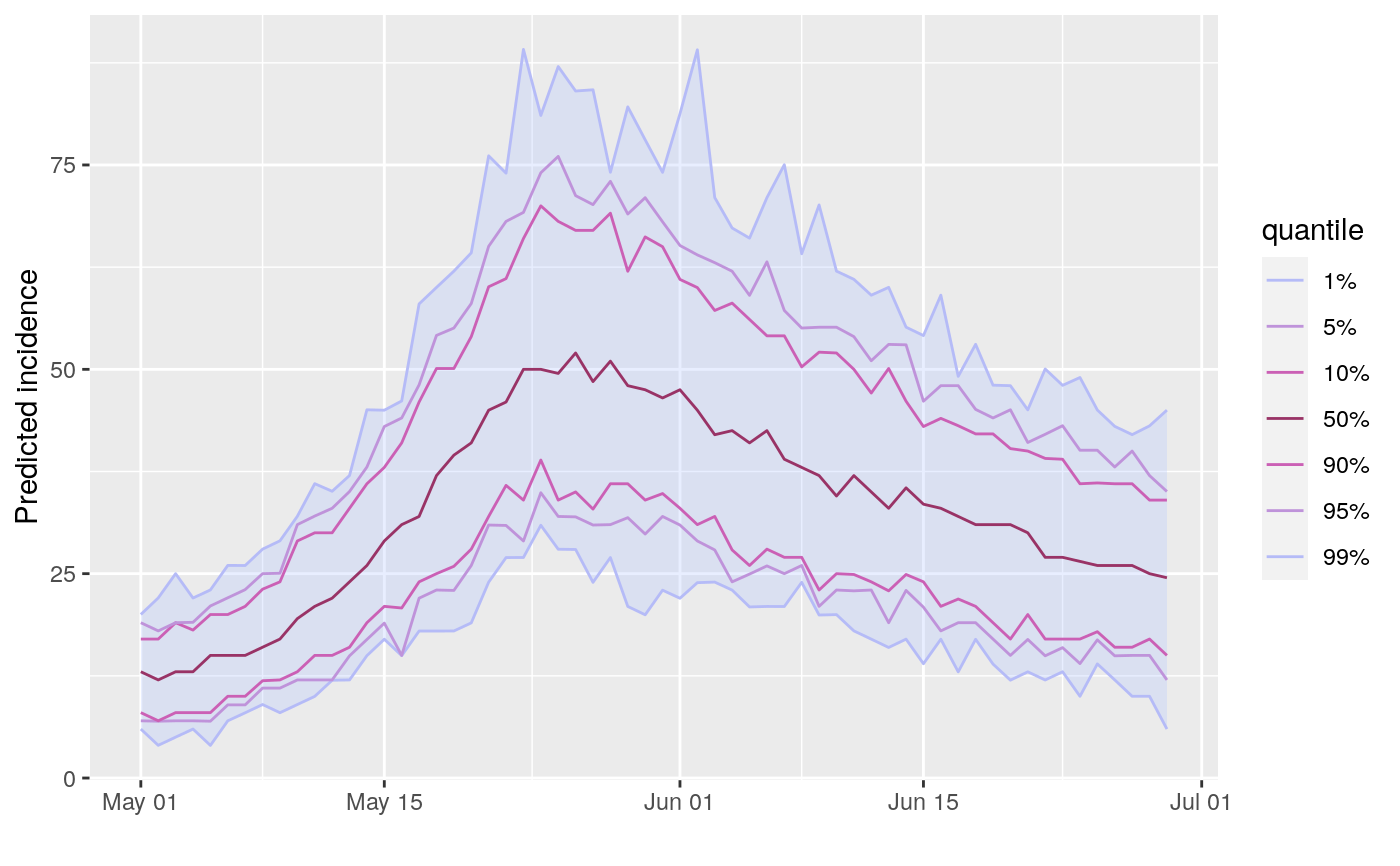
## example using simulated Ebola outbreak if (require(outbreaks) && require(distcrete) && require(incidence) && require(magrittr)) { si <- distcrete("gamma", interval = 1L, shape = 2.4, scale = 4.7, w = 0.5) i <- incidence(ebola_sim$linelist$date_of_onset) plot(i) ## projections after the first 100 days, over 60 days, fixed R to 2.1 set.seed(1) proj_1 <- project(x = i[1:100], R = 2.1, si = si, n_days = 60) plot(proj_1) ## add projections to incidence plot plot(i[1:160]) %>% add_projections(proj_1) ## projections after the first 100 days, over 60 days, ## using a sample of R set.seed(1) R <- rnorm(100, 1.8, 0.2) hist(R, col = "grey", border = "white", main = "Distribution of R") proj_2 <- project(x = i[1:100], R = R, si = si, n_days = 60) ## add projections to incidence plot plot(i[1:160]) %>% add_projections(proj_2) ## same with R constant per simulation (more variability) set.seed(1) proj_3 <- project(x = i[1:100], R = R, si = si, n_days = 60, R_fix_within = TRUE) ## add projections to incidence plot plot(i[1:160]) %>% add_projections(proj_3) ## time-varying R, 2 periods, R is 2.1 then 0.5 set.seed(1) proj_4 <- project(i, R = c(2.1, 0.5), si = si, n_days = 60, time_change = 40, n_sim = 100) plot(proj_4) ## time-varying R, 2 periods, separate distributions of R for each period set.seed(1) R_period_1 <- runif(100, min = 1.1, max = 3) R_period_2 <- runif(100, min = 0.6, max = .9) proj_5 <- project(i, R = list(R_period_1, R_period_2), si = si, n_days = 60, time_change = 20, n_sim = 100) plot(proj_5) }#> #>#> #>#> #>