01 Data Preparation
2018-08-14
epiflows-class.RmdIntroduction
Epiflows can be constructed from two data frames:
-
flows - Each row represents a flow of cases from one location to another This must have at least three columns:
- The location from where the flow originates
- The location where the flow terminates
- The number of cases in the flow (can be an absolute number or estimate)
- locations - Each row represents a different location located in flows with associated metadata. It must have a minimum of one column specifying the location identifier that will match the first two columns of flows.
The metadata in locations such as population size, duration of stay in a given location, date of first and last cases, etc. can be useful in estimating the risk of spread, but not everyone will code their data with identical column names. To facilitate their use in the function estimate_risk_spread(), the epiflows object stores a dictionary of variables in a place called $vars. You can see what variables are stored by default and add varaibles using the global_vars() function:
library("epiflows")
#> epiflows is loaded with the following global variables in `global_vars()`:
#> coordinates, pop_size, duration_stay, first_date, last_date, num_cases
global_vars()
#> [1] "coordinates"   "pop_size"      "duration_stay" "first_date"
#> [5] "last_date"     "num_cases"
When we create our object, we will use these as arguments to tell epiflows which varaibles in our data frame are important.
We have two such data frames containing data from a Yellow Fever outbreak in Brazil (Dorigatti et al., 2017). We will load these examples into our session:
library("epiflows")
data("YF_flows")
data("YF_locations")
head(YF_flows)
#>               from    to         n
#> 1   Espirito Santo Italy  2827.572
#> 2     Minas Gerais Italy 15714.103
#> 3   Rio de Janeiro Italy  8163.938
#> 4        Sao Paulo Italy 34038.681
#> 5 Southeast Brazil Italy 76281.763
#> 6   Espirito Santo Spain  3270.500
YF_locations
#>               location_code location_population num_cases_time_window
#> 1            Espirito Santo             3973697                  2600
#> 2              Minas Gerais            20997560                  4870
#> 3            Rio de Janeiro            16635996                   170
#> 4                 Sao Paulo            44749699                   200
#> 5          Southeast Brazil            86356952                  7840
#> 6                 Argentina                  NA                    NA
#> 7                     Chile                  NA                    NA
#> 8                   Germany                  NA                    NA
#> 9                     Italy                  NA                    NA
#> 10                 Paraguay                  NA                    NA
#> 11                 Portugal                  NA                    NA
#> 12                    Spain                  NA                    NA
#> 13           United Kingdom                  NA                    NA
#> 14 United States of America                  NA                    NA
#> 15                  Uruguay                  NA                    NA
#>    first_date_cases last_date_cases length_of_stay
#> 1        2017-01-04      2017-04-30             NA
#> 2        2016-12-19      2017-04-20             NA
#> 3        2017-02-19      2017-05-10             NA
#> 4        2016-12-17      2017-04-20             NA
#> 5        2016-12-17      2017-05-10             NA
#> 6              <NA>            <NA>           10.9
#> 7              <NA>            <NA>           10.3
#> 8              <NA>            <NA>           22.3
#> 9              <NA>            <NA>           30.1
#> 10             <NA>            <NA>            7.3
#> 11             <NA>            <NA>           27.2
#> 12             <NA>            <NA>           27.2
#> 13             <NA>            <NA>           19.5
#> 14             <NA>            <NA>           18.5
#> 15             <NA>            <NA>            8.0
We want to use these data to estimate the risk of spread to other locations. This can be done with the procedure implemented in the estimate_risk_spread() function, which can take an epiflows object.
Construction of the epiflows object from data frames
With these data frames, we can construct the epiflows object using the make_epiflows() function. Note that this assumes that the required columns (id, from, to, and n) are in the correct order. If they aren’t we can specify their locations with the options in make_epiflows(). Type help("make_epiflows") for more details.
ef <- make_epiflows(flows         = YF_flows,
                    locations     = YF_locations,
                    pop_size      = "location_population",
                    duration_stay = "length_of_stay",
                    num_cases     = "num_cases_time_window",
                    first_date    = "first_date_cases",
                    last_date     = "last_date_cases"
                   )
print(ef)
#>
#> /// Epidemiological Flows //
#>
#>   // class: epiflows, epicontacts
#>   // 15 locations; 100 flows; directed
#>   // optional variables: pop_size, duration_stay, num_cases, first_date, last_date
#>
#>   // locations
#>
#> # A tibble: 15 x 6
#>    id    location_popula… num_cases_time_… first_date_cases last_date_cases
#>  * <chr>            <dbl>            <dbl> <fct>            <fct>
#>  1 Espi…          3973697             2600 2017-01-04       2017-04-30
#>  2 Mina…         20997560             4870 2016-12-19       2017-04-20
#>  3 Rio …         16635996              170 2017-02-19       2017-05-10
#>  4 Sao …         44749699              200 2016-12-17       2017-04-20
#>  5 Sout…         86356952             7840 2016-12-17       2017-05-10
#>  6 Arge…               NA               NA <NA>             <NA>
#>  7 Chile               NA               NA <NA>             <NA>
#>  8 Germ…               NA               NA <NA>             <NA>
#>  9 Italy               NA               NA <NA>             <NA>
#> 10 Para…               NA               NA <NA>             <NA>
#> 11 Port…               NA               NA <NA>             <NA>
#> 12 Spain               NA               NA <NA>             <NA>
#> 13 Unit…               NA               NA <NA>             <NA>
#> 14 Unit…               NA               NA <NA>             <NA>
#> 15 Urug…               NA               NA <NA>             <NA>
#> # ... with 1 more variable: length_of_stay <dbl>
#>
#>   // flows
#>
#> # A tibble: 100 x 3
#>    from             to         n
#>    <chr>            <chr>  <dbl>
#>  1 Espirito Santo   Italy  2828.
#>  2 Minas Gerais     Italy 15714.
#>  3 Rio de Janeiro   Italy  8164.
#>  4 Sao Paulo        Italy 34039.
#>  5 Southeast Brazil Italy 76282.
#>  6 Espirito Santo   Spain  3270.
#>  7 Minas Gerais     Spain 18176.
#>  8 Rio de Janeiro   Spain  9443.
#>  9 Sao Paulo        Spain 39371.
#> 10 Southeast Brazil Spain 88231.
#> # ... with 90 more rows
Now we can use this with esitmate_risk_spread()
incubation <- function(n) {
  rlnorm(n, 1.46, 0.35)
}

infectious <- function(n) {
  rnorm(n, 4.5, 1.5/1.96)
}
set.seed(2017-07-25)
res <- estimate_risk_spread(ef,
                            location_code          = "Espirito Santo",
                            r_incubation           = incubation,
                            r_infectious           = infectious,
                            n_sim                  = 1e5)
#> Exportations done
#> Importations done
res
#>                          mean_cases lower_limit_95CI upper_limit_95CI
#> Italy                     0.2231010        0.1521863        0.3071570
#> Spain                     0.2252568        0.1538359        0.3119207
#> Portugal                  0.2314011        0.1566451        0.3372611
#> Germany                   0.1861744        0.1260291        0.2713440
#> United Kingdom            0.1611980        0.1195965        0.2084865
#> United States of America  0.9241416        0.6255894        1.3469106
#> Argentina                 1.1268870        0.7628361        1.6424064
#> Chile                     0.2644830        0.1790425        0.3854833
#> Uruguay                   0.2405802        0.1628641        0.3506508
#> Paraguay                  0.1618686        0.1213829        0.1924263
We can use ggplot2 to visualize these data
library("ggplot2")
res$location <- factor(rownames(res), rownames(res))
ggplot(res, aes(x = mean_cases, y = location)) +
  geom_point(size = 2) +
  geom_errorbarh(aes(xmin = lower_limit_95CI, xmax = upper_limit_95CI), height = .25) +
  theme_bw(base_size = 12, base_family = "Helvetica") +
  ggtitle("Yellow Fever Spread from Espirito Santo, Brazil") +
  xlab("Number of cases") +
  xlim(c(0, NA))
By default, estimate_risk_spread() returns a summary of the simulations. To obtain the full simulated output, you can set return_all_simulations = TRUE:
set.seed(2017-07-25)
res <- estimate_risk_spread(ef,
                            location_code          = "Espirito Santo",
                            r_incubation           = incubation,
                            r_infectious           = infectious,
                            n_sim                  = 1e5,
                            return_all_simulations = TRUE)
#> Exportations done
#> Importations done
head(res)
#>          Italy     Spain  Portugal   Germany United Kingdom
#> [1,] 0.1881972 0.1902371 0.1937110 0.1558506      0.1454655
#> [2,] 0.1643659 0.1661475 0.1691815 0.1361153      0.1291680
#> [3,] 0.2300272 0.2325205 0.2367666 0.1904910      0.1643677
#> [4,] 0.2479176 0.2506047 0.2551811 0.2053064      0.1724519
#> [5,] 0.2580284 0.2600902 0.2655881 0.2136794      0.1770208
#> [6,] 0.2005721 0.2027461 0.2064485 0.1660986      0.1510575
#>      United States of America Argentina     Chile   Uruguay  Paraguay
#> [1,]                0.7736187 0.9433412 0.2214082 0.2014016 0.1501050
#> [2,]                0.6756559 0.8238866 0.1933715 0.1758983 0.1310973
#> [3,]                0.9455686 1.1530148 0.2706200 0.2461665 0.1665537
#> [4,]                1.0191100 1.2426903 0.2916674 0.2653121 0.1712946
#> [5,]                1.0606723 1.2933709 0.3035624 0.2761323 0.1739739
#> [6,]                0.8244880 1.0053706 0.2359669 0.2146448 0.1587483
library("ggplot2")
ggplot(utils::stack(as.data.frame(res)), aes(x = ind, y = values)) +
  geom_boxplot(outlier.alpha = 0.2) +
  theme_bw(base_size = 12, base_family = "Helvetica") +
  ggtitle("Yellow Fever Spread from Espirito Santo, Brazil") +
  ylab("Number of cases") +
  xlab("Location") +
  ylim(c(0, NA)) +
  coord_flip()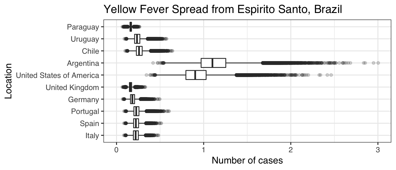
Using set_vars() to update variable keys in the object
In some cases, it may be useful to store several vectors that can represent a single variable in the model and switch them out. These vectors can be stored as separate columns in the data frame and you can use the function set_vars() to change which column a default variable points to.
Example: different durations of stay
data preparation
Such a case may arise if you have several different durations of stay based on the location of origin. For example, let’s imagine that this was the case for the Brazilian data. First, we’ll construct some dummy data.
data("YF_Brazil")
set.seed(5000)
short_stays <- as.data.frame(replicate(5, rpois(10, 5) + round(runif(10), 1)))
colnames(short_stays) <- c("ES", "MG", "RdJ", "SP", "SB")
rownames(short_stays) <- names(YF_Brazil$length_of_stay)
short_stays
#>                            ES  MG RdJ   SP  SB
#> Italy                     5.3 6.6 6.8  7.5 8.6
#> Spain                     5.9 2.2 3.3  6.4 3.6
#> Portugal                  3.9 4.1 3.3 10.5 9.2
#> Germany                  10.6 6.5 8.1  7.8 6.8
#> United Kingdom            1.1 4.1 4.1  3.1 7.1
#> United States of America  6.6 5.3 3.0  3.4 3.5
#> Argentina                 7.5 6.4 5.7  5.3 6.6
#> Chile                     1.2 6.8 0.8  4.5 2.7
#> Uruguay                   4.9 8.9 5.6  3.5 7.8
#> Paraguay                  5.2 3.4 5.0  4.9 4.3
Now, we can merge it with our original locations metadata using the location_code column to join the two together correctly:
short_stays$location_code <- rownames(short_stays)
(locations <- merge(YF_locations, short_stays, by = "location_code", all = TRUE, sort = FALSE))
#>               location_code location_population num_cases_time_window
#> 1                 Argentina                  NA                    NA
#> 2                     Chile                  NA                    NA
#> 3                   Germany                  NA                    NA
#> 4                     Italy                  NA                    NA
#> 5                  Paraguay                  NA                    NA
#> 6                  Portugal                  NA                    NA
#> 7                     Spain                  NA                    NA
#> 8            United Kingdom                  NA                    NA
#> 9  United States of America                  NA                    NA
#> 10                  Uruguay                  NA                    NA
#> 11           Espirito Santo             3973697                  2600
#> 12             Minas Gerais            20997560                  4870
#> 13           Rio de Janeiro            16635996                   170
#> 14                Sao Paulo            44749699                   200
#> 15         Southeast Brazil            86356952                  7840
#>    first_date_cases last_date_cases length_of_stay   ES  MG RdJ   SP  SB
#> 1              <NA>            <NA>           10.9  7.5 6.4 5.7  5.3 6.6
#> 2              <NA>            <NA>           10.3  1.2 6.8 0.8  4.5 2.7
#> 3              <NA>            <NA>           22.3 10.6 6.5 8.1  7.8 6.8
#> 4              <NA>            <NA>           30.1  5.3 6.6 6.8  7.5 8.6
#> 5              <NA>            <NA>            7.3  5.2 3.4 5.0  4.9 4.3
#> 6              <NA>            <NA>           27.2  3.9 4.1 3.3 10.5 9.2
#> 7              <NA>            <NA>           27.2  5.9 2.2 3.3  6.4 3.6
#> 8              <NA>            <NA>           19.5  1.1 4.1 4.1  3.1 7.1
#> 9              <NA>            <NA>           18.5  6.6 5.3 3.0  3.4 3.5
#> 10             <NA>            <NA>            8.0  4.9 8.9 5.6  3.5 7.8
#> 11       2017-01-04      2017-04-30             NA   NA  NA  NA   NA  NA
#> 12       2016-12-19      2017-04-20             NA   NA  NA  NA   NA  NA
#> 13       2017-02-19      2017-05-10             NA   NA  NA  NA   NA  NA
#> 14       2016-12-17      2017-04-20             NA   NA  NA  NA   NA  NA
#> 15       2016-12-17      2017-05-10             NA   NA  NA  NA   NA  NA
Now we can create the epiflows object like we did before, but using our added data:
ef <- make_epiflows(flows         = YF_flows,
                    locations     = locations,
                    pop_size      = "location_population",
                    duration_stay = "length_of_stay",
                    num_cases     = "num_cases_time_window",
                    first_date    = "first_date_cases",
                    last_date     = "last_date_cases"
                   )
Using set_vars()
We can run the model the same, but now we have the option to switch out which columns from our locations data frame we want to use:
get_vars(ef)$duration_stay
#> [1] "length_of_stay"
set_vars(ef, "duration_stay") <- "ES"
get_vars(ef)$duration_stay
#> [1] "ES"
set.seed(2017-07-25)
incubation <- function(n) {
  rlnorm(n, 1.46, 0.35)
}

infectious <- function(n) {
  rnorm(n, 4.5, 1.5/1.96)
}
set.seed(2017-07-25)
res <- estimate_risk_spread(ef,
                            location_code          = "Espirito Santo",
                            r_incubation           = incubation,
                            r_infectious           = infectious,
                            n_sim                  = 1e5)
#> Exportations done
#> Importations done
res$location <- factor(rownames(res), rownames(res))
ggplot(res, aes(x = mean_cases, y = location)) +
  geom_point(size = 2) +
  geom_errorbarh(aes(xmin = lower_limit_95CI, xmax = upper_limit_95CI), height = .25) +
  theme_bw(base_size = 12, base_family = "Helvetica") +
  ggtitle("Yellow Fever Spread from Espirito Santo, Brazil") +
  xlab("Number of cases") +
  xlim(c(0, NA))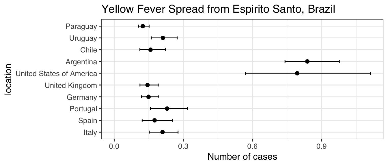
Changing it back is simple:
set_vars(ef, "duration_stay") <- "length_of_stay"

set.seed(2017-07-25)
res <- estimate_risk_spread(ef,
                            location_code          = "Espirito Santo",
                            r_incubation           = incubation,
                            r_infectious           = infectious,
                            n_sim                  = 1e5)
#> Exportations done
#> Importations done
res$location <- factor(rownames(res), rownames(res))
ggplot(res, aes(x = mean_cases, y = location)) +
  geom_point(size = 2) +
  geom_errorbarh(aes(xmin = lower_limit_95CI, xmax = upper_limit_95CI), height = .25) +
  theme_bw(base_size = 12, base_family = "Helvetica") +
  ggtitle("Yellow Fever Spread from Espirito Santo, Brazil") +
  xlab("Number of cases") +
  xlim(c(0, NA))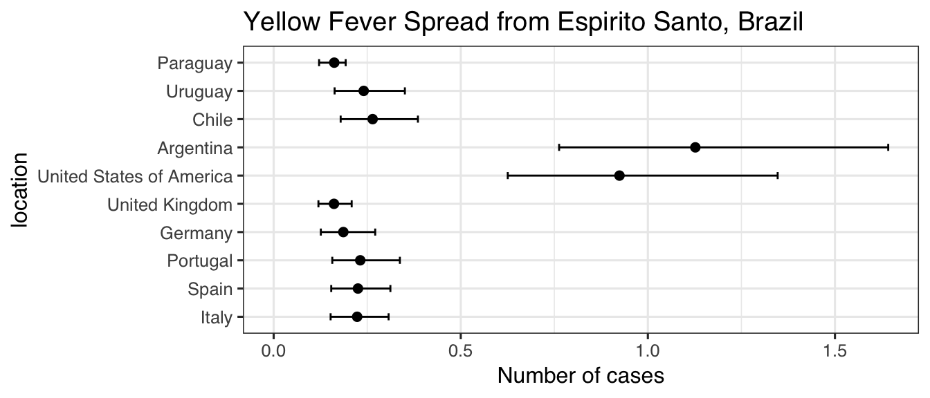
Using a custom argument
Or, you can specify it by adding it as an argument in the function
set.seed(2017-07-25)
res <- estimate_risk_spread(ef,
                            location_code          = "Espirito Santo",
                            r_incubation           = incubation,
                            r_infectious           = infectious,
                            n_sim                  = 1e5,
                            avg_length_stay_days   = rep(2, 10))
#> Exportations done
#> Importations done
res$location <- factor(rownames(res), rownames(res))
ggplot(res, aes(x = mean_cases, y = location)) +
  geom_point(size = 2) +
  geom_errorbarh(aes(xmin = lower_limit_95CI, xmax = upper_limit_95CI), height = .25) +
  theme_bw(base_size = 12, base_family = "Helvetica") +
  ggtitle("Yellow Fever Spread from Espirito Santo, Brazil") +
  xlab("Number of cases") +
  xlim(c(0, NA))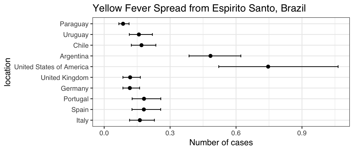
References
Dorigatti I, Hamlet A, Aguas R, Cattarino L, Cori A, Donnelly CA, Garske T, Imai N, Ferguson NM. International risk of yellow fever spread from the ongoing outbreak in Brazil, December 2016 to May 2017. Euro Surveill. 2017;22(28):pii=30572. DOI: 10.2807/1560-7917.ES.2017.22.28.30572