00 epiflows: package overview
2018-08-14
introduction.Rmdepiflows is a package for predicting and visualising spread of infectious diseases based on flows between geographical locations, e.g., countries. epiflows provides functions for calculating spread estimates, handling flow data, and visualization.
Installing the package
Currently, epiflows is a work in progress and can be installed from github using the remotes, ghit, or devtools package:
if (!require("remotes")) install.packages("remotes", repos = "https://cloud.rstudio.org")
remotes::install_github("reconhub/epiflows")
What does it do?
The main features of the package include:
Estimation of risk
-
estimate_risk_spread(): calculate estimates (point estimate and 95% CI) for disease spread from flow data
Example
Estimating the number of new cases flowing to other countries from Espirito Santo, Brazil (Dorigatti et al., 2017).
library("epiflows")## epiflows is loaded with the following global variables in `global_vars()`:
## coordinates, pop_size, duration_stay, first_date, last_date, num_caseslibrary("ggplot2")
data("Brazil_epiflows")
print(Brazil_epiflows)##
## /// Epidemiological Flows //
##
## // class: epiflows, epicontacts
## // 15 locations; 100 flows; directed
## // optional variables: pop_size, duration_stay, num_cases, first_date, last_date
##
## // locations
##
## # A tibble: 15 x 6
## id location_popula… num_cases_time_… first_date_cases last_date_cases
## * <chr> <dbl> <dbl> <fct> <fct>
## 1 Espi… 3973697 2600 2017-01-04 2017-04-30
## 2 Mina… 20997560 4870 2016-12-19 2017-04-20
## 3 Rio … 16635996 170 2017-02-19 2017-05-10
## 4 Sao … 44749699 200 2016-12-17 2017-04-20
## 5 Sout… 86356952 7840 2016-12-17 2017-05-10
## 6 Arge… NA NA <NA> <NA>
## 7 Chile NA NA <NA> <NA>
## 8 Germ… NA NA <NA> <NA>
## 9 Italy NA NA <NA> <NA>
## 10 Para… NA NA <NA> <NA>
## 11 Port… NA NA <NA> <NA>
## 12 Spain NA NA <NA> <NA>
## 13 Unit… NA NA <NA> <NA>
## 14 Unit… NA NA <NA> <NA>
## 15 Urug… NA NA <NA> <NA>
## # ... with 1 more variable: length_of_stay <dbl>
##
## // flows
##
## # A tibble: 100 x 3
## from to n
## <chr> <chr> <dbl>
## 1 Espirito Santo Italy 2828.
## 2 Minas Gerais Italy 15714.
## 3 Rio de Janeiro Italy 8164.
## 4 Sao Paulo Italy 34039.
## 5 Southeast Brazil Italy 76282.
## 6 Espirito Santo Spain 3270.
## 7 Minas Gerais Spain 18176.
## 8 Rio de Janeiro Spain 9443.
## 9 Sao Paulo Spain 39371.
## 10 Southeast Brazil Spain 88231.
## # ... with 90 more rowsset.seed(2018-07-25)
res <- estimate_risk_spread(Brazil_epiflows,
location_code = "Espirito Santo",
r_incubation = function(n) rlnorm(n, 1.46, 0.35),
r_infectious = function(n) rnorm(n, 4.5, 1.5/1.96),
n_sim = 1e5
)## Exportations done## Importations doneres## mean_cases lower_limit_95CI upper_limit_95CI
## Italy 0.2233656 0.1520966 0.3078136
## Spain 0.2255171 0.1537452 0.3126801
## Portugal 0.2317019 0.1565528 0.3383112
## Germany 0.1864162 0.1259548 0.2721890
## United Kingdom 0.1613418 0.1195261 0.2089475
## United States of America 0.9253419 0.6252207 1.3511047
## Argentina 1.1283506 0.7623865 1.6475205
## Chile 0.2648277 0.1789370 0.3866836
## Uruguay 0.2408942 0.1627681 0.3517426
## Paraguay 0.1619724 0.1213114 0.1926966res$location <- rownames(res)
ggplot(res, aes(x = mean_cases, y = location)) +
geom_point(size = 2) +
geom_errorbarh(aes(xmin = lower_limit_95CI, xmax = upper_limit_95CI), height = .25) +
theme_bw(base_size = 12, base_family = "Helvetica") +
ggtitle("Yellow Fever Spread from Espirito Santo, Brazil") +
xlab("Number of cases") +
xlim(c(0, NA))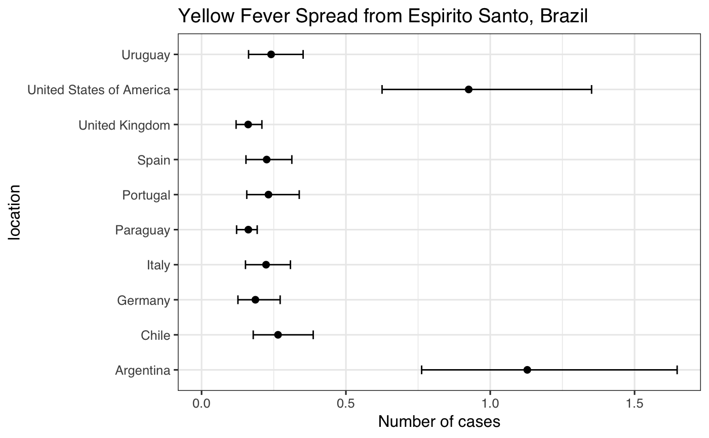
Data structure to store flows and metadata
-
epiflows: an S3 class for storing flow data, as well as country metadata. This class contains two data frames containing flows and location metadata based on theepicontactsclass from the epicontacts pacakge. -
make_epiflows(): a constructor forepiflowsfrom either a pair of data frames or inflows and outflows and location data frame. -
add_coordinates(): add latitude/longitude to the location data in anepiflowsobject usingggmap::geocode()
The easiest way to create an epiflows object is from two data frames (type vignette("epiflows-class") for more details:
data("YF_locations")
data("YF_flows")
data("YF_coordinates")
loc <- merge(x = YF_locations,
             y = YF_coordinates,
             by.x = "location_code",
             by.y = "id",
             sort = FALSE)
loc
## location_code location_population num_cases_time_window
## 1 Espirito Santo 3973697 2600
## 2 Minas Gerais 20997560 4870
## 3 Rio de Janeiro 16635996 170
## 4 Sao Paulo 44749699 200
## 5 Southeast Brazil 86356952 7840
## 6 Argentina NA NA
## 7 Chile NA NA
## 8 Germany NA NA
## 9 Italy NA NA
## 10 Paraguay NA NA
## 11 Portugal NA NA
## 12 Spain NA NA
## 13 United Kingdom NA NA
## 14 United States of America NA NA
## 15 Uruguay NA NA
## first_date_cases last_date_cases length_of_stay lon lat
## 1 2017-01-04 2017-04-30 NA -40.308863 -19.18342
## 2 2016-12-19 2017-04-20 NA -44.555031 -18.51218
## 3 2017-02-19 2017-05-10 NA -43.172897 -22.90685
## 4 2016-12-17 2017-04-20 NA -46.633309 -23.55052
## 5 2016-12-17 2017-05-10 NA -46.209155 -20.33318
## 6 <NA> <NA> 10.9 -63.616672 -38.41610
## 7 <NA> <NA> 10.3 -71.542969 -35.67515
## 8 <NA> <NA> 22.3 10.451526 51.16569
## 9 <NA> <NA> 30.1 12.567380 41.87194
## 10 <NA> <NA> 7.3 -58.443832 -23.44250
## 11 <NA> <NA> 27.2 -8.224454 39.39987
## 12 <NA> <NA> 27.2 -3.749220 40.46367
## 13 <NA> <NA> 19.5 -3.435973 55.37805
## 14 <NA> <NA> 18.5 -95.712891 37.09024
## 15 <NA> <NA> 8.0 -55.765835 -32.52278ef <- make_epiflows(flows = YF_flows,
locations = loc,
coordinates = c("lon", "lat"),
pop_size = "location_population",
duration_stay = "length_of_stay",
num_cases = "num_cases_time_window",
first_date = "first_date_cases",
last_date = "last_date_cases"
)
ef##
## /// Epidemiological Flows //
##
## // class: epiflows, epicontacts
## // 15 locations; 100 flows; directed
## // optional variables: coordinates, pop_size, duration_stay, num_cases, first_date, last_date
##
## // locations
##
## # A tibble: 15 x 8
## id location_popula… num_cases_time_… first_date_cases last_date_cases
## * <chr> <dbl> <dbl> <fct> <fct>
## 1 Espi… 3973697 2600 2017-01-04 2017-04-30
## 2 Mina… 20997560 4870 2016-12-19 2017-04-20
## 3 Rio … 16635996 170 2017-02-19 2017-05-10
## 4 Sao … 44749699 200 2016-12-17 2017-04-20
## 5 Sout… 86356952 7840 2016-12-17 2017-05-10
## 6 Arge… NA NA <NA> <NA>
## 7 Chile NA NA <NA> <NA>
## 8 Germ… NA NA <NA> <NA>
## 9 Italy NA NA <NA> <NA>
## 10 Para… NA NA <NA> <NA>
## 11 Port… NA NA <NA> <NA>
## 12 Spain NA NA <NA> <NA>
## 13 Unit… NA NA <NA> <NA>
## 14 Unit… NA NA <NA> <NA>
## 15 Urug… NA NA <NA> <NA>
## # ... with 3 more variables: length_of_stay <dbl>, lon <dbl>, lat <dbl>
##
## // flows
##
## # A tibble: 100 x 3
## from to n
## <chr> <chr> <dbl>
## 1 Espirito Santo Italy 2828.
## 2 Minas Gerais Italy 15714.
## 3 Rio de Janeiro Italy 8164.
## 4 Sao Paulo Italy 34039.
## 5 Southeast Brazil Italy 76282.
## 6 Espirito Santo Spain 3270.
## 7 Minas Gerais Spain 18176.
## 8 Rio de Janeiro Spain 9443.
## 9 Sao Paulo Spain 39371.
## 10 Southeast Brazil Spain 88231.
## # ... with 90 more rowsBasic methods
-
x[j = myLocations]: subset anepiflowsobject to location(s) myLocations and all that it(they) interact(s) with. -
print(): print summary for anepiflowsobject
Plotting
You can use plot() to plot flows from an epiflows object on one of:
-
leaflet world map (default if coordinates; standalone function:
map_epiflows()) - a visNetwork interactive graph (default if no coordinates; standalone function:
vis_epiflows()) - a grid/bubble plot (standalone function:
grid_epiflows()).
vis_epiflows(ef)map_epiflows(ef)grid_epiflows(ef)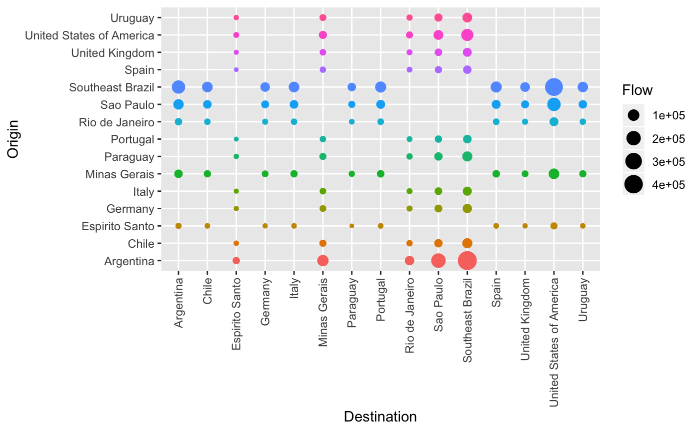
Accessors
-
get_flows(): return flow data -
get_locations(): return metadata for all locations -
get_vars(): access variables from metadata -
get_coordinates(): return coordinates for each location (if provided) -
get_id(): return a vector of location identifiers -
get_n(): return the number of cases per flow -
get_pop_size(): return the population size for each location (if provided)
References
Dorigatti I, Hamlet A, Aguas R, Cattarino L, Cori A, Donnelly CA, Garske T, Imai N, Ferguson NM. International risk of yellow fever spread from the ongoing outbreak in Brazil, December 2016 to May 2017. Euro Surveill. 2017;22(28):pii=30572. DOI: 10.2807/1560-7917.ES.2017.22.28.30572