Introduction
occupancy implements forecasting of daily bed occupancy using input data on both daily hospital admissions and the density distribution for the duration of stay. It aims to provide a reliable and standardised approach to forecasting that will help improve the quality and ease of provision of predictions.
Available functions
occupancy contains three functions:
-
project_bedsis the main function to compute projections of bed occupancy from admissions data and a length of stay distribution. -
build_projectionsis reexported from theprojectionspackage. It allows the user to build a object that can be fed to theproject_bedsfunction. -
incidenceis reexported from theincidencepackage. Similarly to thebuild_projectionsfunction above, it allows the user to build a object that can be fed toproject_beds.
Usage
library(occupancy)
library(ggplot2)    # for plotting
library(scales)     # for plotting
library(distcrete)  # for disretisation
We consider two examples where we have hospital admission data and our goal is to predict bed occupancy for the following weeks. With both examples we will consider an outbreak in it’s early stages, where we anticipate exponential growth in the number of cases.
Both examples will use a Weibull distribution for length of stay and the distcrete package to discretise the distribution.
length_of_stay <-
    distcrete("weibull", shape = 1.1, scale = 7.4, w = 0.5, interval = 1)
Example 1
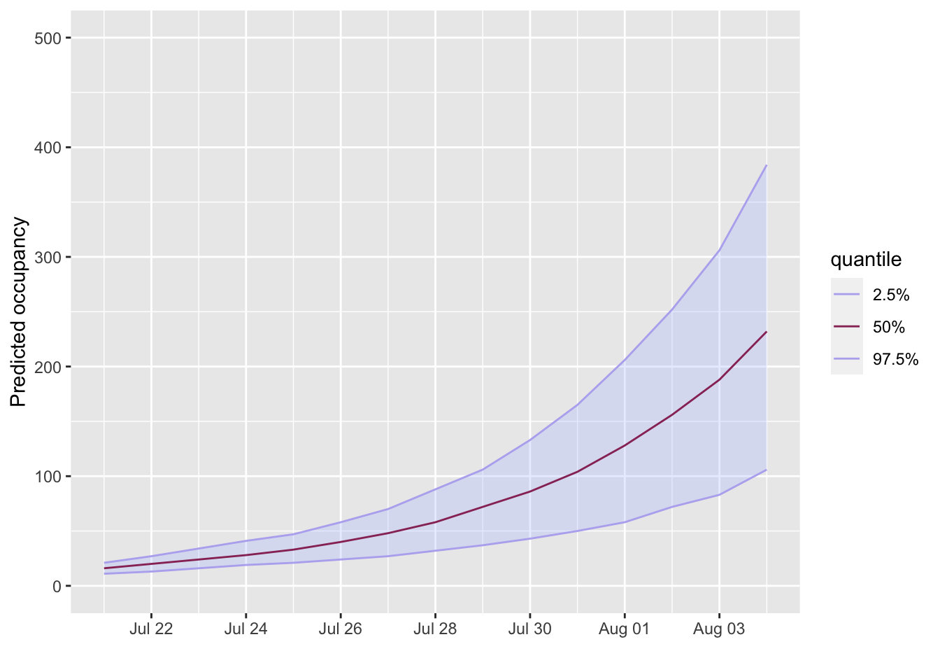
In this example we assume the disease has a doubling time of 7 days and that there are initially 10 hospital admissions.
initial_admissions <- 10 # day one
duration <- 14           # 14 days (2 weeks) duration
growth_rate <- log(2) / 7 # doubling time of 7 days

future_admissions <- round(
    initial_admissions * exp(growth_rate * (seq_len(duration))))

admissions <-
  incidence(rep(Sys.Date() + 0:14, c(initial_admissions, future_admissions)))

# convert to a projections object to use with the project_beds function
admissions <- build_projections(
    x = c(initial_admissions, future_admissions),
    dates = Sys.Date() + 0:14)
We now have all the variables we need to make our forecast of bed occupancy
projection <- project_beds(x = admissions,
                           r_los = length_of_stay,
                           n_sims = 10)

plot(projection, quantiles = c(0.025, 0.5), ylab = "Predicted occupancy") +
    scale_x_date(breaks = breaks_pretty(10)) +
    ylim(0, 500)
#> Scale for 'x' is already present. Adding another scale for 'x', which will
#> replace the existing scale.
Example 2
In this example we assume we have a weeks worth of admission data that, again, we want to forecast the next 14 days. This time, however, we would like to encorporate the serial-interval of the disease as well as an estimation of R0.
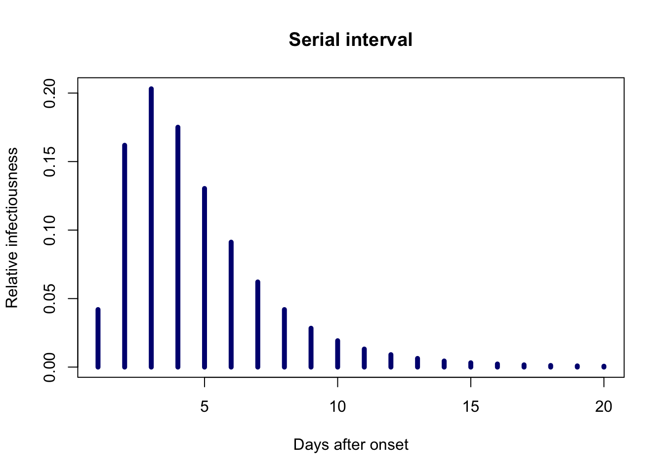
To start with we make up some toy admissions data and create a discretised serial interval. To give the example some some grounding in reality we use some reasearch from the recent COVID-19 pandemic. In a small study it was observed that a log-normal distribution provided a good fit for data that had an observed mean of 4.7 days and standard deviation of 2.9 days. In what follows we use a value of R0 = 2.5.
library(projections)  # so we can use the `project` and subset functions

# make some fake admissions data
initial_admissions <- sample(Sys.Date() - 0:7, 30, replace = TRUE)
initial_admissions <- incidence(initial_admissions)

# observed study values need converting before use with R's log-normal function
recorded_mean <- 4.7
recorded_sd <- 2.9
mu <- log(recorded_mean^2 / sqrt(recorded_mean^2 + recorded_sd^2))
sd <- sqrt(log(1 + recorded_sd^2 / recorded_mean^2))

# generate the discretised serial inteval
serial_interval <- distcrete("lnorm", mu, sd, w = 0.5, interval = 1)
plot(1:20, serial_interval$d(1:20), type = "h", lwd = 5, col = "navy",
     main = "Serial interval", xlab = "Days after onset",
     ylab = "Relative infectiousness")
# project future admissions
future_admissions <- project(initial_admissions,
                             R = c(2,2.5), si = serial_interval,
                             n_days = 14, n_sim = 100)

# combine the current and future admissions data
original_admissions <- build_projections(initial_admissions$counts,
                                        initial_admissions$dates)
admissions <- future_admissions + original_admissions
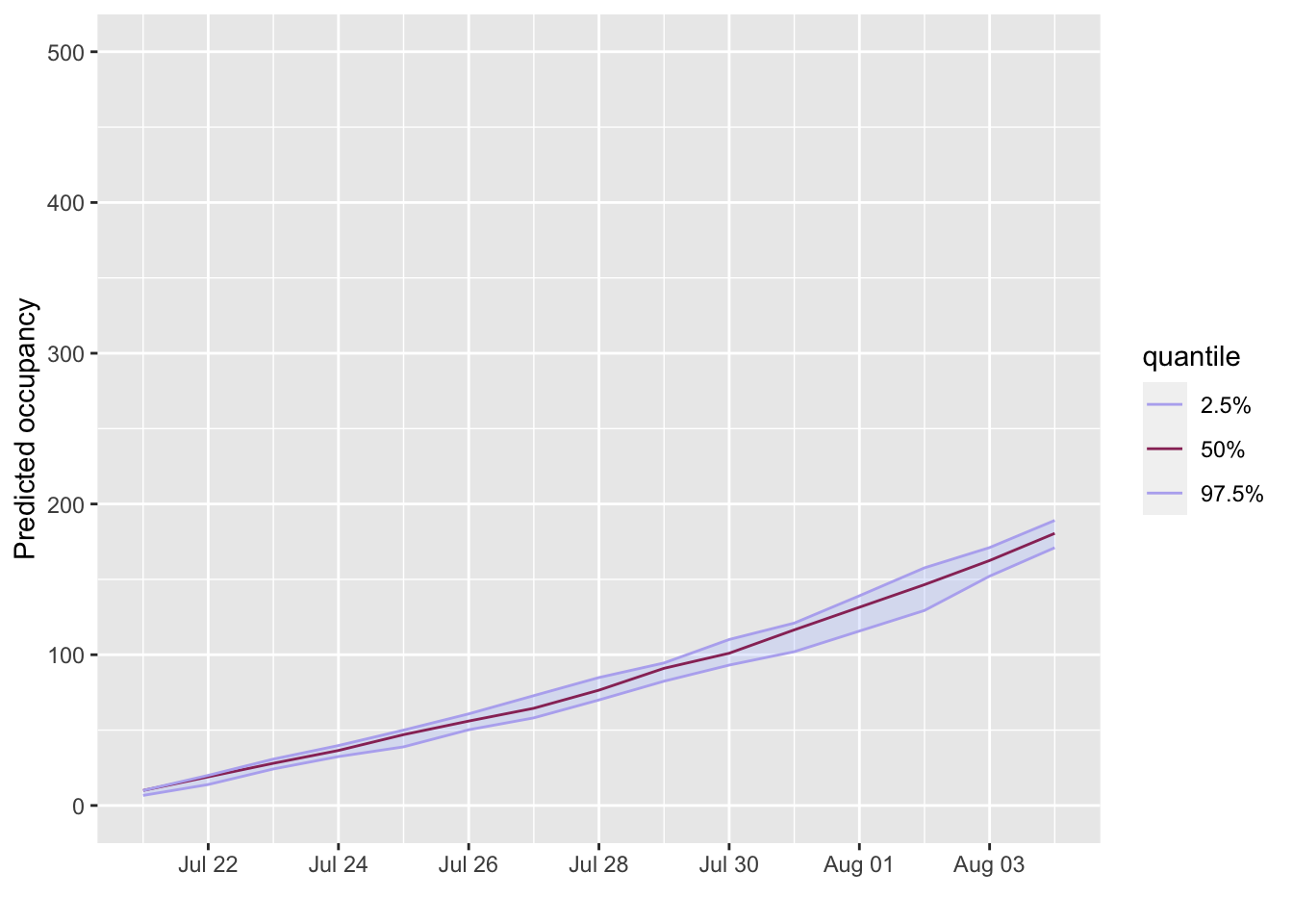
Now we can again make our forecasts
projections <- project_beds(x = admissions,
                           r_los = length_of_stay,
                           n_sims = 10)

projections <- subset(projections, from = Sys.Date())

plot(projections, quantiles = c(0.025, 0.5), ylab = "Predicted occupancy") +
    scale_x_date(breaks = breaks_pretty(10)) +
    ylim(0, 500)
#> Scale for 'x' is already present. Adding another scale for 'x', which will
#> replace the existing scale.