Details of the incidence class
Thibaut Jombart, Zhian N. Kamvar
2025-06-19
Source:vignettes/incidence_class.Rmd
incidence_class.RmdThis vignette details the structure of incidence objects, as
produced by the incidence function.
Structure of an incidence object.
We generate a toy dataset of dates to examine the content of incidence objects.
library(incidence)
set.seed(1)
dat <- sample(1:50, 200, replace = TRUE, prob = 1 + exp(1:50 * 0.1))
sex <- sample(c("female", "male"), 200, replace = TRUE)
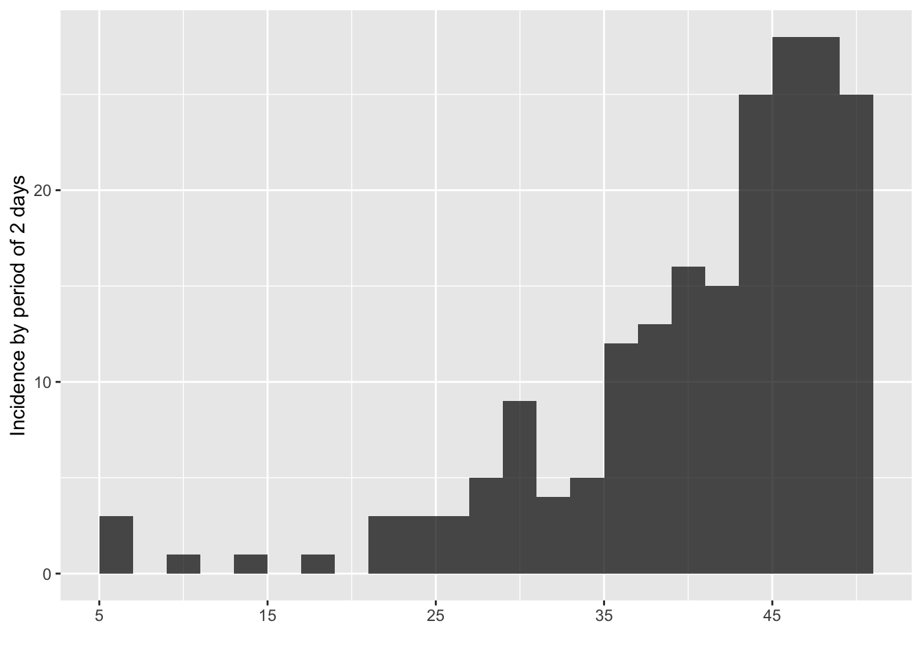
The incidence by 48h period is computed as:
i <- incidence(dat, interval = 2)
i
#> <incidence object>
#> [200 cases from days 5 to 49]
#>
#> $counts: matrix with 23 rows and 1 columns
#> $n: 200 cases in total
#> $dates: 23 dates marking the left-side of bins
#> $interval: 2 days
#> $timespan: 45 days
#> $cumulative: FALSE
plot(i)
#> Warning: `aes_string()` was deprecated in ggplot2 3.0.0.
#> ℹ Please use tidy evaluation idioms with `aes()`.
#> ℹ See also `vignette("ggplot2-in-packages")` for more information.
#> ℹ The deprecated feature was likely used in the incidence package.
#>   Please report the issue at <https://github.com/reconhub/incidence/issues>.
#> This warning is displayed once every 8 hours.
#> Call `lifecycle::last_lifecycle_warnings()` to see where this warning was
#> generated.
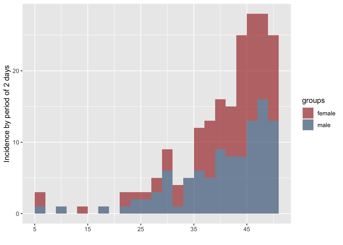
We also compute incidence by gender:
i.sex <- incidence(dat, interval = 2, group = sex)
i.sex
#> <incidence object>
#> [200 cases from days 5 to 49]
#> [2 groups: female, male]
#>
#> $counts: matrix with 23 rows and 2 columns
#> $n: 200 cases in total
#> $dates: 23 dates marking the left-side of bins
#> $interval: 2 days
#> $timespan: 45 days
#> $cumulative: FALSE
plot(i.sex)
The object i is a list with the class
incidence:
class(i)
#> [1] "incidence"
is.list(i)
#> [1] TRUE
names(i)
#> [1] "dates"      "counts"     "timespan"   "interval"   "n"
#> [6] "cumulative"
Items in i can be accessed using the same indexing as
any lists, but it’s safer to use the accessors for each item:
In the following sections, we examine each of the components of the object.
$dates
The $dates component contains a vector for all the dates
for which incidence have been computed, in the format of the input
dataset (e.g. Date, numeric,
integer).
date_bins <- get_dates(i)
class(date_bins)
#> [1] "integer"
class(dat)
#> [1] "integer"

date_bins
#>  [1]  5  7  9 11 13 15 17 19 21 23 25 27 29 31 33 35 37 39 41 43 45 47 49
The dates correspond to the lower bounds of the time intervals used as bins for the incidence. Bins always include the lower bound and exclude the upper bound. In the example provided above, this means that the first bin counts events that happened at day 5-6, the second bin counts events from 7-8, etc.
Note that if we had actual Date-class dates, they would
be returned as dates
dat_Date <- as.Date("2018-10-31") + dat
head(dat_Date)
#> [1] "2018-12-17" "2018-12-16" "2018-12-12" "2018-11-26" "2018-12-18"
#> [6] "2018-11-27"
i.date <- incidence(dat_Date, interval = 2, group = sex)
i.date
#> <incidence object>
#> [200 cases from days 2018-11-05 to 2018-12-19]
#> [2 groups: female, male]
#>
#> $counts: matrix with 23 rows and 2 columns
#> $n: 200 cases in total
#> $dates: 23 dates marking the left-side of bins
#> $interval: 2 days
#> $timespan: 45 days
#> $cumulative: FALSE
get_dates(i.date)
#>  [1] "2018-11-05" "2018-11-07" "2018-11-09" "2018-11-11" "2018-11-13"
#>  [6] "2018-11-15" "2018-11-17" "2018-11-19" "2018-11-21" "2018-11-23"
#> [11] "2018-11-25" "2018-11-27" "2018-11-29" "2018-12-01" "2018-12-03"
#> [16] "2018-12-05" "2018-12-07" "2018-12-09" "2018-12-11" "2018-12-13"
#> [21] "2018-12-15" "2018-12-17" "2018-12-19"
class(get_dates(i.date))
#> [1] "Date"
These can be converted to integers, counting the number of days from the first date.
get_dates(i.date, count_days = TRUE)
#>  [1]  0  2  4  6  8 10 12 14 16 18 20 22 24 26 28 30 32 34 36 38 40 42 44
get_dates(i, count_days = TRUE)
#>  [1]  0  2  4  6  8 10 12 14 16 18 20 22 24 26 28 30 32 34 36 38 40 42 44
To facilitate modelling, it’s also possible to get the center of the
interval by using the position = "center" argument:
get_dates(i.date, position = "center")
#>  [1] "2018-11-06" "2018-11-08" "2018-11-10" "2018-11-12" "2018-11-14"
#>  [6] "2018-11-16" "2018-11-18" "2018-11-20" "2018-11-22" "2018-11-24"
#> [11] "2018-11-26" "2018-11-28" "2018-11-30" "2018-12-02" "2018-12-04"
#> [16] "2018-12-06" "2018-12-08" "2018-12-10" "2018-12-12" "2018-12-14"
#> [21] "2018-12-16" "2018-12-18" "2018-12-20"
get_dates(i.date, position = "center", count_days = TRUE)
#>  [1]  1  3  5  7  9 11 13 15 17 19 21 23 25 27 29 31 33 35 37 39 41 43 45
$counts
The $counts component contains the actual incidence,
i.e. counts of events for the defined bins. It is a matrix
of integers where rows correspond to time intervals, with
one column for each group for which incidence is computed (a single,
unnamed column if no groups were provided). If groups were provided,
columns are named after the groups. We illustrate the difference
comparing the two objects i and i.sex:
counts <- get_counts(i)
class(counts)
#> [1] "matrix" "array"
storage.mode(counts)
#> [1] "integer"

counts
#>       [,1]
#>  [1,]    3
#>  [2,]    0
#>  [3,]    1
#>  [4,]    0
#>  [5,]    1
#>  [6,]    0
#>  [7,]    1
#>  [8,]    0
#>  [9,]    3
#> [10,]    3
#> [11,]    3
#> [12,]    5
#> [13,]    9
#> [14,]    4
#> [15,]    5
#> [16,]   12
#> [17,]   13
#> [18,]   16
#> [19,]   15
#> [20,]   25
#> [21,]   28
#> [22,]   28
#> [23,]   25
get_counts(i.sex)
#>       female male
#>  [1,]      2    1
#>  [2,]      0    0
#>  [3,]      0    1
#>  [4,]      0    0
#>  [5,]      1    0
#>  [6,]      0    0
#>  [7,]      0    1
#>  [8,]      0    0
#>  [9,]      2    1
#> [10,]      1    2
#> [11,]      1    2
#> [12,]      2    3
#> [13,]      3    6
#> [14,]      3    1
#> [15,]      0    5
#> [16,]      6    6
#> [17,]      8    5
#> [18,]      7    9
#> [19,]      7    8
#> [20,]     17    8
#> [21,]     15   13
#> [22,]     12   16
#> [23,]     12   13
You can see the dimensions of the incidence object by using
dim(), ncol(), and nrow(), which
returns the dimensions of the counts matrix:
dim(get_counts(i.sex))
#> [1] 23  2
dim(i.sex)
#> [1] 23  2
nrow(i.sex) # number of date bins
#> [1] 23
ncol(i.sex) # number of groups
#> [1] 2
There are also accessors for handling groups:
# Number of groups
ncol(i.sex)
#> [1] 2
ncol(i)
#> [1] 1

# Names of groups
group_names(i.sex)
#> [1] "female" "male"
group_names(i)
#> NULL

# You can also rename the groups
group_names(i.sex) <- c("F", "M")
group_names(i.sex)
#> [1] "F" "M"
Note that a data.frame containing dates and
counts can be obtained using as.data.frame:
## basic conversion
as.data.frame(i)
#>    dates counts
#> 1      5      3
#> 2      7      0
#> 3      9      1
#> 4     11      0
#> 5     13      1
#> 6     15      0
#> 7     17      1
#> 8     19      0
#> 9     21      3
#> 10    23      3
#> 11    25      3
#> 12    27      5
#> 13    29      9
#> 14    31      4
#> 15    33      5
#> 16    35     12
#> 17    37     13
#> 18    39     16
#> 19    41     15
#> 20    43     25
#> 21    45     28
#> 22    47     28
#> 23    49     25
as.data.frame(i.sex)
#>    dates  F  M
#> 1      5  2  1
#> 2      7  0  0
#> 3      9  0  1
#> 4     11  0  0
#> 5     13  1  0
#> 6     15  0  0
#> 7     17  0  1
#> 8     19  0  0
#> 9     21  2  1
#> 10    23  1  2
#> 11    25  1  2
#> 12    27  2  3
#> 13    29  3  6
#> 14    31  3  1
#> 15    33  0  5
#> 16    35  6  6
#> 17    37  8  5
#> 18    39  7  9
#> 19    41  7  8
#> 20    43 17  8
#> 21    45 15 13
#> 22    47 12 16
#> 23    49 12 13

## long format for ggplot2
as.data.frame(i.sex, long = TRUE)
#>    dates counts groups
#> 1      5      2      F
#> 2      7      0      F
#> 3      9      0      F
#> 4     11      0      F
#> 5     13      1      F
#> 6     15      0      F
#> 7     17      0      F
#> 8     19      0      F
#> 9     21      2      F
#> 10    23      1      F
#> 11    25      1      F
#> 12    27      2      F
#> 13    29      3      F
#> 14    31      3      F
#> 15    33      0      F
#> 16    35      6      F
#> 17    37      8      F
#> 18    39      7      F
#> 19    41      7      F
#> 20    43     17      F
#> 21    45     15      F
#> 22    47     12      F
#> 23    49     12      F
#> 24     5      1      M
#> 25     7      0      M
#> 26     9      1      M
#> 27    11      0      M
#> 28    13      0      M
#> 29    15      0      M
#> 30    17      1      M
#> 31    19      0      M
#> 32    21      1      M
#> 33    23      2      M
#> 34    25      2      M
#> 35    27      3      M
#> 36    29      6      M
#> 37    31      1      M
#> 38    33      5      M
#> 39    35      6      M
#> 40    37      5      M
#> 41    39      9      M
#> 42    41      8      M
#> 43    43      8      M
#> 44    45     13      M
#> 45    47     16      M
#> 46    49     13      M
Note that incidence has an argument called
na_as_group which is TRUE by default, which
will pool all missing groups into a separate group, in which case it
will be a separate column in $counts.
$timespan
The $timespan component stores the length of the time
period covered by the object:
get_timespan(i)
#> [1] 45
print(date_range <- range(get_dates(i)))
#> [1]  5 49
diff(date_range) + 1
#> [1] 45
$interval
The $interval component contains the length of the time
interval for the bins:
get_interval(i)
#> [1] 2
diff(get_dates(i))
#>  [1] 2 2 2 2 2 2 2 2 2 2 2 2 2 2 2 2 2 2 2 2 2 2
$n
The $n component stores the total number of events in
the data:
get_n(i)
#> [1] 200
Note that to obtain the number of cases by groups, one can use:
colSums(get_counts(i.sex))
#>   F   M
#>  99 101
$weeks
The $weeks component is optional, and used to store aweek objects
whenever they have been used. Weeks are used by default when weekly
incidence is computed from dates (see argument standard in
?incidence).
library(outbreaks)
dat <- ebola_sim$linelist$date_of_onset
i.7 <- incidence(dat, "1 epiweek", standard = TRUE)
i.7
#> <incidence object>
#> [5888 cases from days 2014-04-06 to 2015-04-26]
#> [5888 cases from MMWR weeks 2014-W15 to 2015-W17]
#>
#> $counts: matrix with 56 rows and 1 columns
#> $n: 5888 cases in total
#> $dates: 56 dates marking the left-side of bins
#> $interval: 1 week
#> $timespan: 386 days
#> $cumulative: FALSE
i.7$weeks
#> <aweek start: Sunday>
#>  [1] "2014-W15" "2014-W16" "2014-W17" "2014-W18" "2014-W19" "2014-W20"
#>  [7] "2014-W21" "2014-W22" "2014-W23" "2014-W24" "2014-W25" "2014-W26"
#> [13] "2014-W27" "2014-W28" "2014-W29" "2014-W30" "2014-W31" "2014-W32"
#> [19] "2014-W33" "2014-W34" "2014-W35" "2014-W36" "2014-W37" "2014-W38"
#> [25] "2014-W39" "2014-W40" "2014-W41" "2014-W42" "2014-W43" "2014-W44"
#> [31] "2014-W45" "2014-W46" "2014-W47" "2014-W48" "2014-W49" "2014-W50"
#> [37] "2014-W51" "2014-W52" "2014-W53" "2015-W01" "2015-W02" "2015-W03"
#> [43] "2015-W04" "2015-W05" "2015-W06" "2015-W07" "2015-W08" "2015-W09"
#> [49] "2015-W10" "2015-W11" "2015-W12" "2015-W13" "2015-W14" "2015-W15"
#> [55] "2015-W16" "2015-W17"
Because $weeks is an optional element, it does not have
a dedicated accessor. If the element is not present, attempting to
access it will result in a NULL:
i$weeks
#> NULL
Both dates and weeks are returned when converting an
incidence object to data.frame:
head(as.data.frame(i.7))
#>        dates    weeks counts
#> 1 2014-04-06 2014-W15      1
#> 2 2014-04-13 2014-W16      1
#> 3 2014-04-20 2014-W17      4
#> 4 2014-04-27 2014-W18      4
#> 5 2014-05-04 2014-W19     12
#> 6 2014-05-11 2014-W20     15