Details of the incidence_fit class
Zhian N. Kamvar
2025-06-19
Source:vignettes/incidence_fit_class.Rmd
incidence_fit_class.RmdThis vignette details the structure and construction of the
incidence_fit and incidence_fit_list classes,
which are produced by the fit() and
fit_optim_split() functions, respectively. By the end of
this tutorial, you should be able to construct
incidence_fit and incidence_fit_list objects
for use with your own models.
Structure of an incidence_fit object
An incidence_fit object contains three elements:
-
$model: The model fit to anincidenceobject. Currently, this represents a log-linear model, but it can be any model. -
$info: Information derived from the model-
rThe growth rate -
r.confthe confidence interval ofr -
preda data frame containing the predictions of the model using the true dates (dates), their numeric version used in the model (dates.x), the predicted value (fit), and the lower (lwr) and upper (upr) bounds of the associated confidence interval. -
doublingthe predicted doubling time in days (only ifris positive) -
doubling.confthe confidence interval of the doubling time -
halvingthe predicted halving time in days (only ifris negative) -
halving.confthe confidence interval of the halving time
-
-
$origin: the date corresponding to day ‘0’
Internally, when fit() is run, these elements are
constructed by function incidence:::extract_info(). First
we need to setup data. We will use simulated Ebola outbreak data from
the outbreaks package over weekly intervals and calculate the
fit for the first 20 weeks:
library(outbreaks)
library(incidence)
dat <- ebola_sim$linelist$date_of_onset
i <- incidence(dat, interval = "week")
i
#> <incidence object>
#> [5888 cases from days 2014-04-07 to 2015-04-27]
#> [5888 cases from ISO weeks 2014-W15 to 2015-W18]
#>
#> $counts: matrix with 56 rows and 1 columns
#> $n: 5888 cases in total
#> $dates: 56 dates marking the left-side of bins
#> $interval: 1 week
#> $timespan: 386 days
#> $cumulative: FALSE
f <- fit(i[1:20])
f
#> <incidence_fit object>
#>
#> $model: regression of log-incidence over time
#>
#> $info: list containing the following items:
#>   $r (daily growth rate):
#> [1] 0.03175771
#>
#>   $r.conf (confidence interval):
#>           2.5 %     97.5 %
#> [1,] 0.02596229 0.03755314
#>
#>   $doubling (doubling time in days):
#> [1] 21.8261
#>
#>   $doubling.conf (confidence interval):
#>         2.5 %   97.5 %
#> [1,] 18.45777 26.69823
#>
#>   $pred: data.frame of incidence predictions (20 rows, 5 columns)
plot(i, fit = f)
#> Warning: `aes_string()` was deprecated in ggplot2 3.0.0.
#> ℹ Please use tidy evaluation idioms with `aes()`.
#> ℹ See also `vignette("ggplot2-in-packages")` for more information.
#> ℹ The deprecated feature was likely used in the incidence package.
#>   Please report the issue at <https://github.com/reconhub/incidence/issues>.
#> This warning is displayed once every 8 hours.
#> Call `lifecycle::last_lifecycle_warnings()` to see where this warning was
#> generated.
As you can see, the incidence_fit object has a print
method and a plot method. If you want to access individual elements in
the $info element, you can use the get_info()
function:
get_info(f, "r")
#> [1] 0.03175771
get_info(f, "r.conf")
#>           2.5 %     97.5 %
#> [1,] 0.02596229 0.03755314
get_info(f, "doubling.conf")
#>         2.5 %   97.5 %
#> [1,] 18.45777 26.69823
This will be important later when we combine several
incidence_fit objects into a single
incidence_fit_list.
Building an incidence_fit object from scratch
The incidence_fit object can be constructed from any
model from which you can derive the daily growth rate, doubling/halving
times, predictions, and confidence intervals. The following three steps
show roughly how it is done from model fitting to construction.
Step 1: create the model
The default model for fit() is a log-linear model on the
intervals between dates. To fit this model, we will need to create a
data frame with the counts and the midpoints of the intervals:
# ensure all dates have at least one incidence
i2 <- i[1:20]
i2 <- i2[apply(get_counts(i2), 1, min) > 0]
df <- as.data.frame(i2, long = TRUE)
df$dates.x <- get_dates(i2, position = "center", count_days = TRUE)
head(df)
#>        dates    weeks isoweeks counts dates.x
#> 1 2014-04-07 2014-W15 2014-W15      1     3.5
#> 2 2014-04-14 2014-W16 2014-W16      1    10.5
#> 3 2014-04-21 2014-W17 2014-W17      5    17.5
#> 4 2014-04-28 2014-W18 2014-W18      4    24.5
#> 5 2014-05-05 2014-W19 2014-W19     12    31.5
#> 6 2014-05-12 2014-W20 2014-W20     18    38.5
lm1 <- stats::lm(log(counts) ~ dates.x, data = df)
lm1
#>
#> Call:
#> stats::lm(formula = log(counts) ~ dates.x, data = df)
#>
#> Coefficients:
#> (Intercept)      dates.x
#>     0.81660      0.03176
If we compare that to the $model element produced from
fit(), we can see that it is identical:
all.equal(f$model, lm1)
#> [1] TRUE
Step 2: creation of the $info list:
The $info list is created directly from the model
itself:
r <- stats::coef(lm1)["dates.x"]
r.conf <- stats::confint(lm1, "dates.x", 0.95)
new.data <- data.frame(dates.x = sort(unique(lm1$model$dates.x)))
pred     <- exp(stats::predict(lm1, newdata = new.data, interval = "confidence",
                               level = 0.95))
pred <- cbind.data.frame(new.data, pred)
info_list <- list(
  r = r,
  r.conf = r.conf,
  doubling = log(2) / r,
  doubling.conf = log(2) / r.conf,
  pred = pred
)
info_list
#> $r
#>    dates.x
#> 0.03175771
#>
#> $r.conf
#>              2.5 %     97.5 %
#> dates.x 0.02596229 0.03755314
#>
#> $doubling
#> dates.x
#> 21.8261
#>
#> $doubling.conf
#>            2.5 %   97.5 %
#> dates.x 26.69823 18.45777
#>
#> $pred
#>    dates.x        fit        lwr        upr
#> 1      3.5   2.528815   1.611099   3.969283
#> 2     10.5   3.158367   2.082082   4.791013
#> 3     17.5   3.944645   2.687383   5.790104
#> 4     24.5   4.926668   3.463102   7.008763
#> 5     31.5   6.153167   4.453513   8.501484
#> 6     38.5   7.685004   5.711842  10.339797
#> 7     45.5   9.598194   7.300398  12.619220
#> 8     52.5  11.987674   9.289763  15.469105
#> 9     59.5  14.972017  11.757263  19.065771
#> 10    66.5  18.699315  14.786028  23.648299
#> 11    73.5  23.354529  18.467024  29.535566
#> 12    80.5  29.168662  22.905640  37.144163
#> 13    87.5  36.430229  28.231348  47.010209
#> 14    94.5  45.499570  34.607028  59.820534
#> 15   101.5  56.826734  42.236196  76.457588
#> 16   108.5  70.973805  51.369116  98.060497
#> 17   115.5  88.642805  62.309665 126.104782
#> 18   122.5 110.710519  75.424156 162.505217
#> 19   129.5 138.272012  91.152689 209.748604
#> 20   136.5 172.694966 110.023332 271.065700
Step 3: combine lists and create object
the last step is to combine everything into a list and create the object.
origin <- min(get_dates(i2))
info_list$pred$dates <- origin + info_list$pred$dates.x
the_fit <- list(
  lm = lm1,
  info = info_list,
  origin = min(get_dates(i2))
)
class(the_fit) <- "incidence_fit"
the_fit
#> <incidence_fit object>
#>
#> $model: regression of log-incidence over time
#>
#> $info: list containing the following items:
#>   $r (daily growth rate):
#>    dates.x
#> 0.03175771
#>
#>   $r.conf (confidence interval):
#>              2.5 %     97.5 %
#> dates.x 0.02596229 0.03755314
#>
#>   $doubling (doubling time in days):
#> dates.x
#> 21.8261
#>
#>   $doubling.conf (confidence interval):
#>            2.5 %   97.5 %
#> dates.x 26.69823 18.45777
#>
#>   $pred: data.frame of incidence predictions (20 rows, 5 columns)
plot(i, fit = the_fit)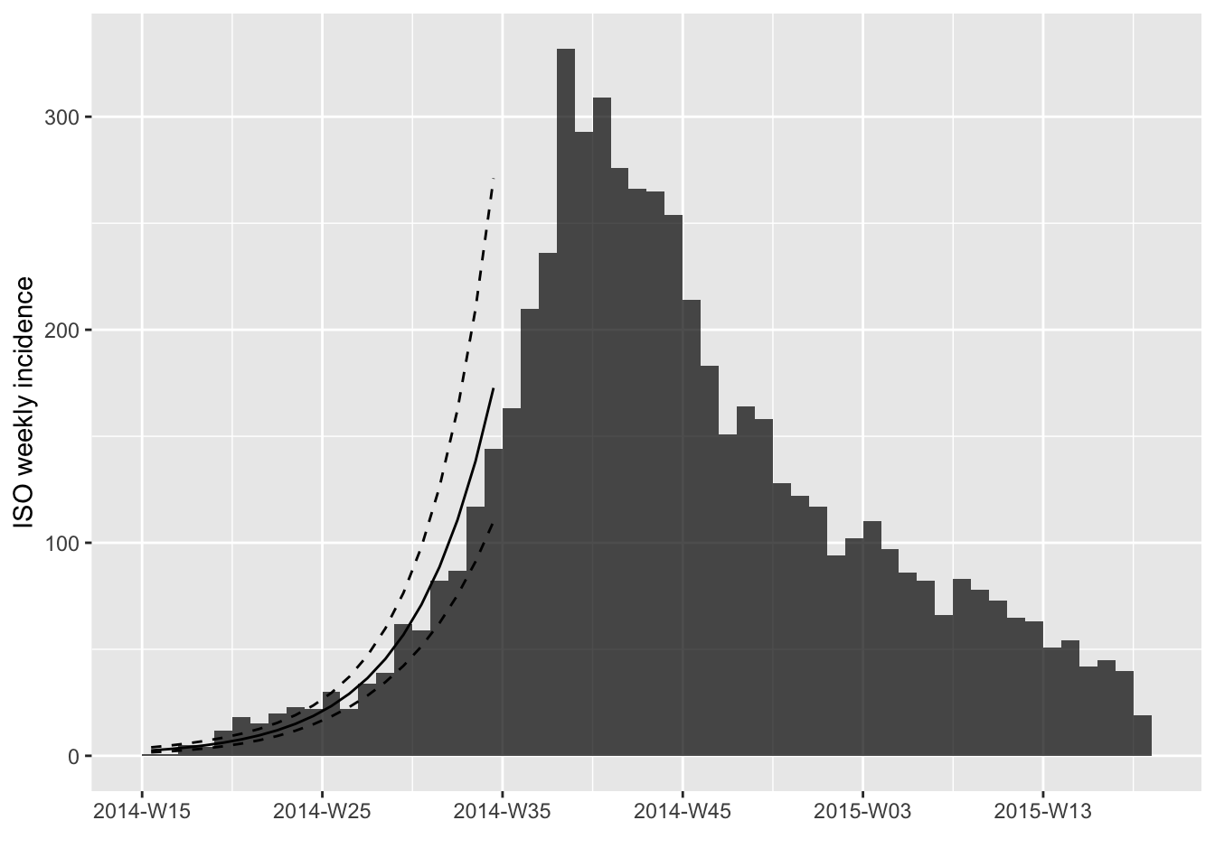
Structure of an incidence_fit_list object
There are several reasons for having multiple fits to a single
incidence object. One may want to have a separate fit for
different groups represented in the object, or one may want to split the
fits at the peak of the epidemic. To aid in plotting and summarizing the
different fits, we’ve created the incidence_fit_list class.
This class has two defining features:
- It consists of a named list containing one or more
incidence_fitobjects or lists containingincidence_fitobjects. - An attribute called “locations” contains a list whose length is
equal to the number of
incidence_fitobjects in the object. Each list element contains a vector that defines where anincidence_fitobject is within theincidence_fit_list.
The reason for this structure is because it is sometimes necessary to
nest lists of incidence_fit objects within lists. When this
happens, accessing individual elements of the objects cumbersome. To
alleviate this, each object has a distinct path within the named list in
the “locations” attribute that allows one to access the object directly
since R allows you to traverse the elements of a nested list by
subsetting with a vector:
l <- list(a = list(b = 1, c = 2),d = list(e = list(f = 3, g = 4), h = 5))
str(l)
#> List of 2
#>  $ a:List of 2
#>   ..$ b: num 1
#>   ..$ c: num 2
#>  $ d:List of 2
#>   ..$ e:List of 2
#>   .. ..$ f: num 3
#>   .. ..$ g: num 4
#>   ..$ h: num 5
l[[c("a", "b")]]
#> [1] 1
l[[c("d", "e", "f")]]
#> [1] 3
Example: A tale of two fits
The function fit_optim_split() attempts to find the
optimal split point in an epicurve, producing an
incidence_fit_list object in the $fit element
of the returned list:
fl <- fit_optim_split(i)
fl$fit
#> <list of incidence_fit objects>
#>
#> attr(x, 'locations'): list of vectors with the locations of each incidence_fit object
#>
#> 'before'
#> 'after'
#>
#> $model: regression of log-incidence over time
#>
#> $info: list containing the following items:
#>   $r (daily growth rate):
#>      before       after
#>  0.02982209 -0.01016191
#>
#>   $r.conf (confidence interval):
#>              2.5 %       97.5 %
#> before  0.02608945  0.033554736
#> after  -0.01102526 -0.009298561
#>
#>   $doubling (doubling time in days):
#>   before
#> 23.24274
#>
#>   $doubling.conf (confidence interval):
#>           2.5 %  97.5 %
#> before 20.65721 26.5681
#>
#>   $halving (halving time in days):
#>    after
#> 68.21031
#>
#>   $halving.conf (confidence interval):
#>          2.5 %   97.5 %
#> after 62.86899 74.54349
#>
#>   $pred: data.frame of incidence predictions (57 rows, 6 columns)
plot(i, fit = fl$fit)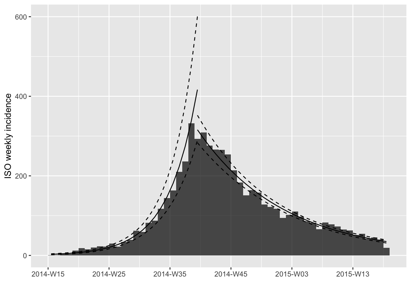
Here you can see that the object looks very similar to the
incidence_fit object, but it has extra information. The
first thing you may notice is the fact that both “doubling” and
“halving” are shown. This is because the two fits have different signs
for the daily growth rate. The second thing you may notice is the fact
that there is something called attr(x, 'locations'). This
attribute gives the location of the incidence_fit objects
within the list. We can illustrate how this works if we look at the
structure of the object:
str(fl$fit, max.level = 2)
#> List of 2
#>  $ before:List of 3
#>   ..$ model :List of 12
#>   .. ..- attr(*, "class")= chr "lm"
#>   ..$ info  :List of 5
#>   ..$ origin: Date[1:1], format: "2014-04-07"
#>   ..- attr(*, "class")= chr "incidence_fit"
#>  $ after :List of 3
#>   ..$ model :List of 12
#>   .. ..- attr(*, "class")= chr "lm"
#>   ..$ info  :List of 5
#>   ..$ origin: Date[1:1], format: "2014-09-22"
#>   ..- attr(*, "class")= chr "incidence_fit"
#>  - attr(*, "locations")=List of 2
#>   ..$ : chr "before"
#>   ..$ : chr "after"
#>  - attr(*, "class")= chr "incidence_fit_list"
Internally, all of the methods for incidence_fit_list
use the ‘locations’ attribute to navigate:
methods(class = "incidence_fit_list")
#> [1] get_fit  get_info plot     print
#> see '?methods' for accessing help and source code
For example, it’s often useful to extract the growth rate for all
models at once. The get_info() method allows us to do this
easily:
get_info(fl$fit, "r")
#>      before       after
#>  0.02982209 -0.01016191
get_info(fl$fit, "r.conf")
#>              2.5 %       97.5 %
#> before  0.02608945  0.033554736
#> after  -0.01102526 -0.009298561
Because doubling or halving is determined by whether or not
r is negative, we automatically filter out the results that
don’t make sense, but you can include them with
na.rm = FALSE:
Example: Nested incidence_fit
Above, we showed the example of a basic
incidence_fit_list class with two objects representing the
fits before and after the peak of an epicurve. However, it is often
useful evaluate fits for different groups separately. Here, we will
construct an incidence object, but define groups by gender:
gen <- ebola_sim$linelist$gender
ig <- incidence(dat, interval = "week", group = gen)
plot(ig, border = "grey98")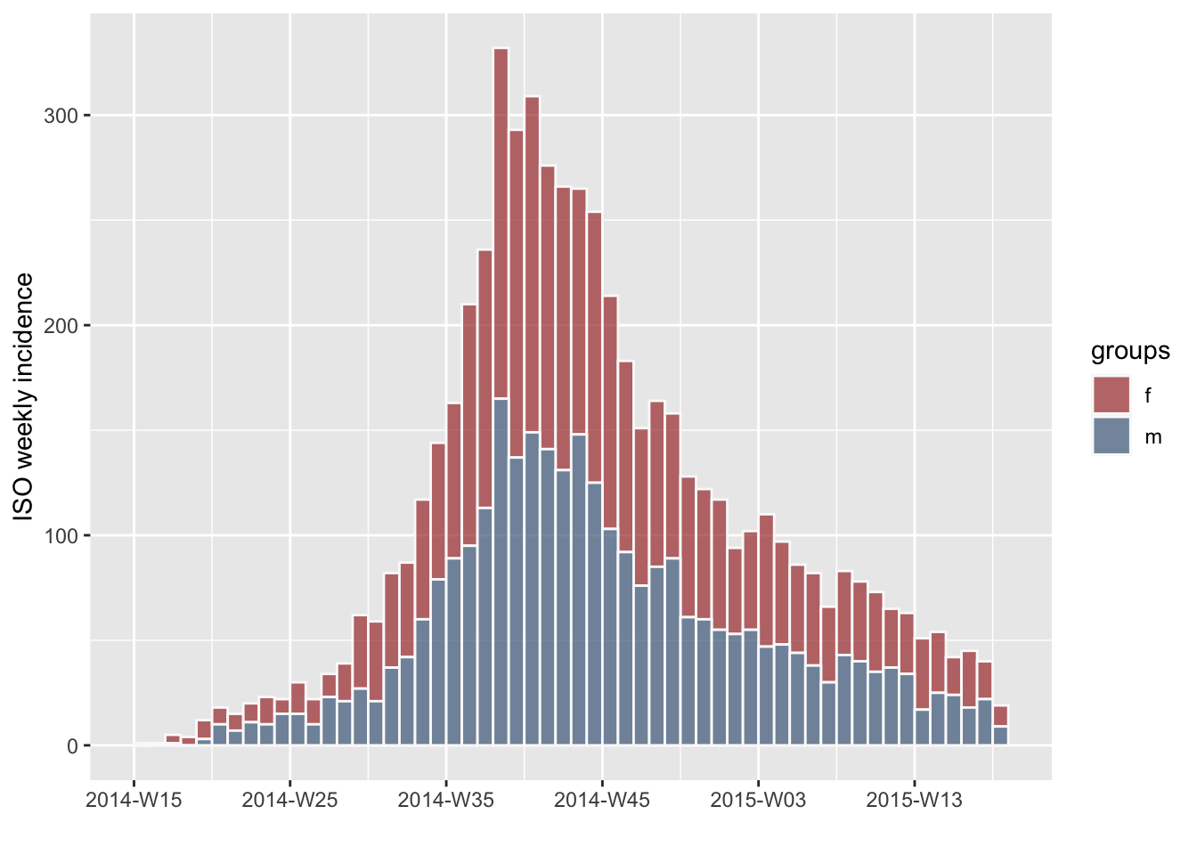
Now if we calculate an optimal fit split, we will end up with four different fits: two for each defined gender.
fg <- fit_optim_split(ig)
plot(ig, fit = fg$fit, border = "grey98", stack = FALSE)
#> Scale for colour is already present.
#> Adding another scale for colour, which will replace the existing scale.
#> Scale for colour is already present.
#> Adding another scale for colour, which will replace the existing scale.
#> Scale for colour is already present.
#> Adding another scale for colour, which will replace the existing scale.
#> Scale for colour is already present.
#> Adding another scale for colour, which will replace the existing scale.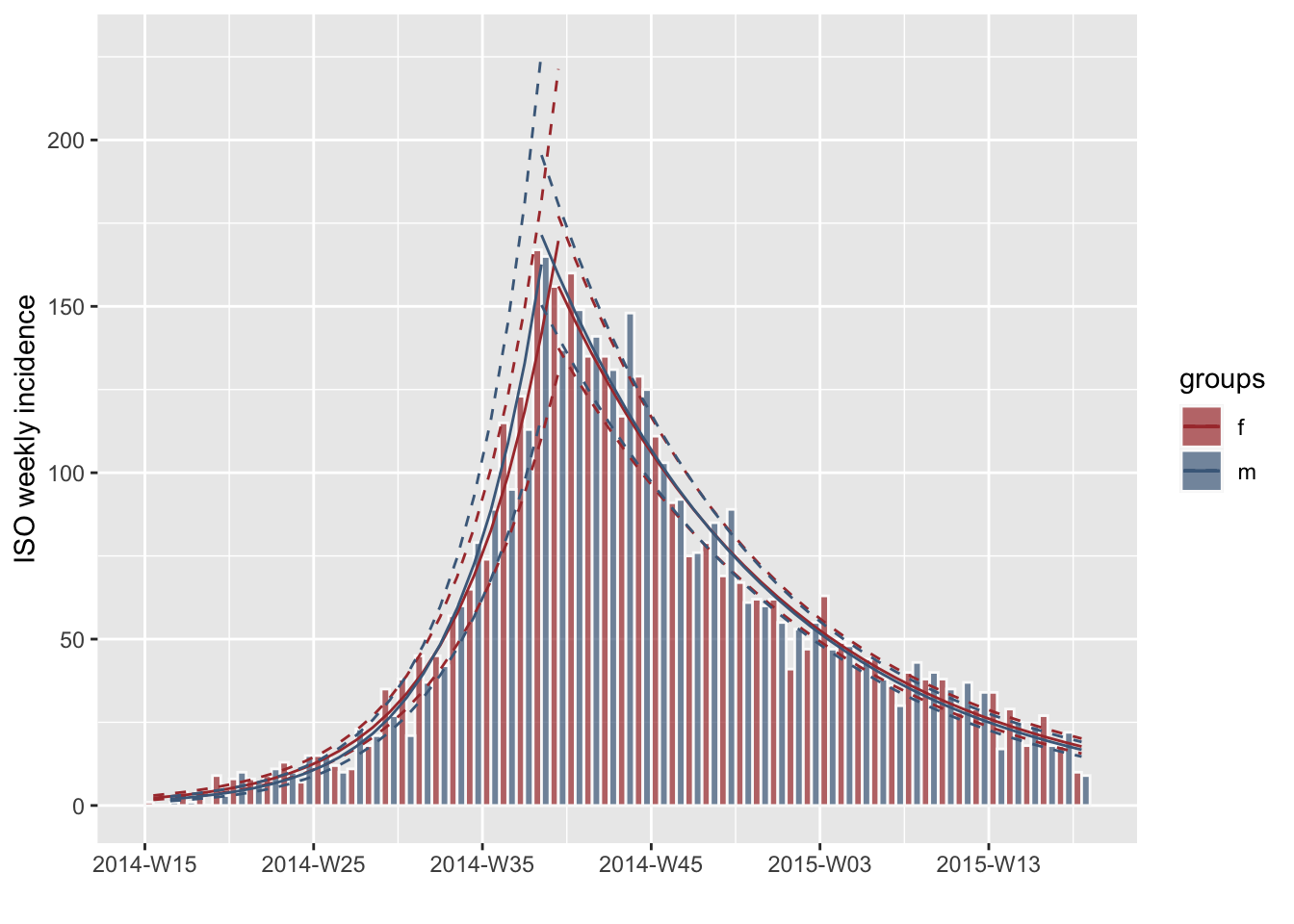
If we look at the fit object, we can see again that it is an
incidence_fit_list but this time with four fits
defined.
fg$fit
#> <list of incidence_fit objects>
#>
#> attr(x, 'locations'): list of vectors with the locations of each incidence_fit object
#>
#> 'f', 'before'
#> 'm', 'before'
#> 'f', 'after'
#> 'm', 'after'
#>
#> $model: regression of log-incidence over time
#>
#> $info: list containing the following items:
#>   $r (daily growth rate):
#>    f_before    m_before     f_after     m_after
#>  0.02570604  0.02883607 -0.01002297 -0.01038307
#>
#>   $r.conf (confidence interval):
#>                2.5 %       97.5 %
#> f_before  0.02289333  0.028518743
#> m_before  0.02502254  0.032649606
#> f_after  -0.01102735 -0.009018595
#> m_after  -0.01138910 -0.009377034
#>
#>   $doubling (doubling time in days):
#> f_before m_before
#> 26.96437 24.03750
#>
#>   $doubling.conf (confidence interval):
#>             2.5 %   97.5 %
#> f_before 24.30497 30.27725
#> m_before 21.22988 27.70091
#>
#>   $halving (halving time in days):
#>  f_after  m_after
#> 69.15586 66.75746
#>
#>   $halving.conf (confidence interval):
#>            2.5 %   97.5 %
#> f_after 62.85711 76.85756
#> m_after 60.86059 73.91966
#>
#>   $pred: data.frame of incidence predictions (111 rows, 7 columns)
str(fg$fit, max.level = 3)
#> List of 2
#>  $ f:List of 2
#>   ..$ before:List of 3
#>   .. ..$ model :List of 12
#>   .. .. ..- attr(*, "class")= chr "lm"
#>   .. ..$ info  :List of 5
#>   .. ..$ origin: Date[1:1], format: "2014-04-07"
#>   .. ..- attr(*, "class")= chr "incidence_fit"
#>   ..$ after :List of 3
#>   .. ..$ model :List of 12
#>   .. .. ..- attr(*, "class")= chr "lm"
#>   .. ..$ info  :List of 5
#>   .. ..$ origin: Date[1:1], format: "2014-09-22"
#>   .. ..- attr(*, "class")= chr "incidence_fit"
#>   ..- attr(*, "locations")=List of 2
#>   .. ..$ : chr "before"
#>   .. ..$ : chr "after"
#>   ..- attr(*, "class")= chr "incidence_fit_list"
#>  $ m:List of 2
#>   ..$ before:List of 3
#>   .. ..$ model :List of 12
#>   .. .. ..- attr(*, "class")= chr "lm"
#>   .. ..$ info  :List of 5
#>   .. ..$ origin: Date[1:1], format: "2014-04-14"
#>   .. ..- attr(*, "class")= chr "incidence_fit"
#>   ..$ after :List of 3
#>   .. ..$ model :List of 12
#>   .. .. ..- attr(*, "class")= chr "lm"
#>   .. ..$ info  :List of 5
#>   .. ..$ origin: Date[1:1], format: "2014-09-15"
#>   .. ..- attr(*, "class")= chr "incidence_fit"
#>   ..- attr(*, "locations")=List of 2
#>   .. ..$ : chr "before"
#>   .. ..$ : chr "after"
#>   ..- attr(*, "class")= chr "incidence_fit_list"
#>  - attr(*, "locations")=List of 4
#>   ..$ : chr [1:2] "f" "before"
#>   ..$ : chr [1:2] "m" "before"
#>   ..$ : chr [1:2] "f" "after"
#>   ..$ : chr [1:2] "m" "after"
#>  - attr(*, "class")= chr "incidence_fit_list"
Notice that the nested lists themselves are of class
incidence_fit_list.
Now, even though the fits within nested lists, the ‘locations’
attributes still defines where they are within the object so that the
get_info() function still operates normally:
get_info(fg$fit, "r.conf")
#>                2.5 %       97.5 %
#> f_before  0.02289333  0.028518743
#> m_before  0.02502254  0.032649606
#> f_after  -0.01102735 -0.009018595
#> m_after  -0.01138910 -0.009377034
If you need to access all the fits easily, a convenience function to
flatten the list is available in get_fit():
str(get_fit(fg$fit), max.level = 2)
#> List of 4
#>  $ f_before:List of 3
#>   ..$ model :List of 12
#>   .. ..- attr(*, "class")= chr "lm"
#>   ..$ info  :List of 5
#>   ..$ origin: Date[1:1], format: "2014-04-07"
#>   ..- attr(*, "class")= chr "incidence_fit"
#>  $ m_before:List of 3
#>   ..$ model :List of 12
#>   .. ..- attr(*, "class")= chr "lm"
#>   ..$ info  :List of 5
#>   ..$ origin: Date[1:1], format: "2014-04-14"
#>   ..- attr(*, "class")= chr "incidence_fit"
#>  $ f_after :List of 3
#>   ..$ model :List of 12
#>   .. ..- attr(*, "class")= chr "lm"
#>   ..$ info  :List of 5
#>   ..$ origin: Date[1:1], format: "2014-09-22"
#>   ..- attr(*, "class")= chr "incidence_fit"
#>  $ m_after :List of 3
#>   ..$ model :List of 12
#>   .. ..- attr(*, "class")= chr "lm"
#>   ..$ info  :List of 5
#>   ..$ origin: Date[1:1], format: "2014-09-15"
#>   ..- attr(*, "class")= chr "incidence_fit"
Because all that defines an incidence_fit_list is the
class definition and the ‘locations’ attribute that defines the
positions of the incidence_fit objects within the nesting,
then it’s also possible to define the output of
fit_optim_split() as an incidence_fit_list
class:
print(locs <- attributes(fg$fit)$locations)
#> [[1]]
#> [1] "f"      "before"
#>
#> [[2]]
#> [1] "m"      "before"
#>
#> [[3]]
#> [1] "f"     "after"
#>
#> [[4]]
#> [1] "m"     "after"

for (i in seq_along(locs)) {
    locs[[i]] <- c("fit", locs[[i]])
}
print(locs)
#> [[1]]
#> [1] "fit"    "f"      "before"
#>
#> [[2]]
#> [1] "fit"    "m"      "before"
#>
#> [[3]]
#> [1] "fit"   "f"     "after"
#>
#> [[4]]
#> [1] "fit"   "m"     "after"
fg.ifl <- fg
attributes(fg.ifl)$locations<- locs
class(fg.ifl) <- "incidence_fit_list"
Now when we print the object, we can see that it prints only the
information related to the incidence_fit_list:
fg.ifl
#> <list of incidence_fit objects>
#>
#> attr(x, 'locations'): list of vectors with the locations of each incidence_fit object
#>
#> 'fit', 'f', 'before'
#> 'fit', 'm', 'before'
#> 'fit', 'f', 'after'
#> 'fit', 'm', 'after'
#>
#> $model: regression of log-incidence over time
#>
#> $info: list containing the following items:
#>   $r (daily growth rate):
#> fit_f_before fit_m_before  fit_f_after  fit_m_after
#>   0.02570604   0.02883607  -0.01002297  -0.01038307
#>
#>   $r.conf (confidence interval):
#>                    2.5 %       97.5 %
#> fit_f_before  0.02289333  0.028518743
#> fit_m_before  0.02502254  0.032649606
#> fit_f_after  -0.01102735 -0.009018595
#> fit_m_after  -0.01138910 -0.009377034
#>
#>   $doubling (doubling time in days):
#> fit_f_before fit_m_before
#>     26.96437     24.03750
#>
#>   $doubling.conf (confidence interval):
#>                 2.5 %   97.5 %
#> fit_f_before 24.30497 30.27725
#> fit_m_before 21.22988 27.70091
#>
#>   $halving (halving time in days):
#> fit_f_after fit_m_after
#>    69.15586    66.75746
#>
#>   $halving.conf (confidence interval):
#>                2.5 %   97.5 %
#> fit_f_after 62.85711 76.85756
#> fit_m_after 60.86059 73.91966
#>
#>   $pred: data.frame of incidence predictions (111 rows, 7 columns)
But, we still retain all of the extra information in the list:
str(fg.ifl, max.level = 1)
#> List of 4
#>  $ df   :'data.frame':   26 obs. of  3 variables:
#>  $ split: Date[1:2], format: "2014-09-22" "2014-09-15"
#>   ..- attr(*, "names")="f" "m"
#>  $ fit  :List of 2
#>   ..- attr(*, "locations")=List of 4
#>   ..- attr(*, "class")= chr "incidence_fit_list"
#>  $ plot : <ggplot2::ggplot>
#>   ..@ data       :'data.frame':  26 obs. of  3 variables:
#>   ..@ layers     :List of 3
#>   ..@ scales     :Classes 'ScalesList', 'ggproto', 'gg' <ggproto object: Class ScalesList, gg>
#>     add: function
#>     add_defaults: function
#>     add_missing: function
#>     backtransform_df: function
#>     clone: function
#>     find: function
#>     get_scales: function
#>     has_scale: function
#>     input: function
#>     map_df: function
#>     n: function
#>     non_position_scales: function
#>     scales: list
#>     set_palettes: function
#>     train_df: function
#>     transform_df: function
#>     super:  <ggproto object: Class ScalesList, gg>
#>   ..@ guides     :Classes 'Guides', 'ggproto', 'gg' <ggproto object: Class Guides, gg>
#>     add: function
#>     assemble: function
#>     build: function
#>     draw: function
#>     get_custom: function
#>     get_guide: function
#>     get_params: function
#>     get_position: function
#>     guides: NULL
#>     merge: function
#>     missing: <ggproto object: Class GuideNone, Guide, gg>
#>         add_title: function
#>         arrange_layout: function
#>         assemble_drawing: function
#>         available_aes: any
#>         build_decor: function
#>         build_labels: function
#>         build_ticks: function
#>         build_title: function
#>         draw: function
#>         draw_early_exit: function
#>         elements: list
#>         extract_decor: function
#>         extract_key: function
#>         extract_params: function
#>         get_layer_key: function
#>         hashables: list
#>         measure_grobs: function
#>         merge: function
#>         override_elements: function
#>         params: list
#>         process_layers: function
#>         setup_elements: function
#>         setup_params: function
#>         train: function
#>         transform: function
#>         super:  <ggproto object: Class GuideNone, Guide, gg>
#>     package_box: function
#>     print: function
#>     process_layers: function
#>     setup: function
#>     subset_guides: function
#>     train: function
#>     update_params: function
#>     super:  <ggproto object: Class Guides, gg>
#>   ..@ mapping    : <ggplot2::mapping> List of 3
#>  .. .. $ colour: language ~groups
#>  .. ..  ..- attr(*, ".Environment")=<environment: 0x555fefa2b1e8>
#>  .. .. $ x     : language ~dates
#>  .. ..  ..- attr(*, ".Environment")=<environment: 0x555fefa2b1e8>
#>  .. .. $ y     : language ~mean.R2
#>  .. ..  ..- attr(*, ".Environment")=<environment: 0x555fefa2b1e8>
#>   ..@ theme      : <theme>  Named list()
#>  .. .. @ complete: logi FALSE
#>  .. .. @ validate: logi TRUE
#>   ..@ coordinates:Classes 'CoordCartesian', 'Coord', 'ggproto', 'gg' <ggproto object: Class CoordCartesian, Coord, gg>
#>     aspect: function
#>     backtransform_range: function
#>     clip: on
#>     default: TRUE
#>     distance: function
#>     draw_panel: function
#>     expand: TRUE
#>     is_free: function
#>     is_linear: function
#>     labels: function
#>     limits: list
#>     modify_scales: function
#>     range: function
#>     ratio: NULL
#>     render_axis_h: function
#>     render_axis_v: function
#>     render_bg: function
#>     render_fg: function
#>     reverse: none
#>     setup_data: function
#>     setup_layout: function
#>     setup_panel_guides: function
#>     setup_panel_params: function
#>     setup_params: function
#>     train_panel_guides: function
#>     transform: function
#>     super:  <ggproto object: Class CoordCartesian, Coord, gg>
#>   ..@ facet      :Classes 'FacetNull', 'Facet', 'ggproto', 'gg' <ggproto object: Class FacetNull, Facet, gg>
#>     attach_axes: function
#>     attach_strips: function
#>     compute_layout: function
#>     draw_back: function
#>     draw_front: function
#>     draw_labels: function
#>     draw_panel_content: function
#>     draw_panels: function
#>     finish_data: function
#>     format_strip_labels: function
#>     init_gtable: function
#>     init_scales: function
#>     map_data: function
#>     params: list
#>     set_panel_size: function
#>     setup_data: function
#>     setup_panel_params: function
#>     setup_params: function
#>     shrink: TRUE
#>     train_scales: function
#>     vars: function
#>     super:  <ggproto object: Class FacetNull, Facet, gg>
#>   ..@ layout     :Classes 'Layout', 'ggproto', 'gg' <ggproto object: Class Layout, gg>
#>     coord: NULL
#>     coord_params: list
#>     facet: NULL
#>     facet_params: list
#>     finish_data: function
#>     get_scales: function
#>     layout: NULL
#>     map_position: function
#>     panel_params: NULL
#>     panel_scales_x: NULL
#>     panel_scales_y: NULL
#>     render: function
#>     render_labels: function
#>     reset_scales: function
#>     resolve_label: function
#>     setup: function
#>     setup_panel_guides: function
#>     setup_panel_params: function
#>     train_position: function
#>     super:  <ggproto object: Class Layout, gg>
#>   ..@ labels     : <ggplot2::labels>  Named list()
#>   ..@ meta       : list()
#>   ..@ plot_env   :<environment: 0x555fefa2b1e8>
#>  - attr(*, "locations")=List of 4
#>  - attr(*, "class")= chr "incidence_fit_list"
fg.ifl$split
#>            f            m
#> "2014-09-22" "2014-09-15"
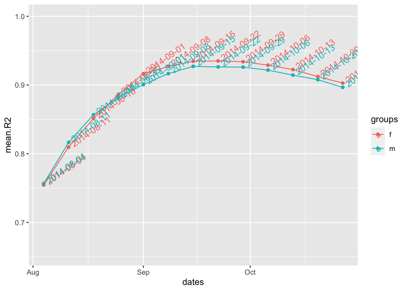
fg.ifl$df
#>         dates   mean.R2 groups
#> 1  2014-08-04 0.7546016      f
#> 2  2014-08-11 0.8096672      f
#> 3  2014-08-18 0.8513743      f
#> 4  2014-08-25 0.8864424      f
#> 5  2014-09-01 0.9165063      f
#> 6  2014-09-08 0.9270248      f
#> 7  2014-09-15 0.9345352      f
#> 8  2014-09-22 0.9350323      f
#> 9  2014-09-29 0.9339121      f
#> 10 2014-10-06 0.9288956      f
#> 11 2014-10-13 0.9226037      f
#> 12 2014-10-20 0.9122727      f
#> 13 2014-10-27 0.9027890      f
#> 14 2014-08-04 0.7566712      m
#> 15 2014-08-11 0.8164693      m
#> 16 2014-08-18 0.8567850      m
#> 17 2014-08-25 0.8820669      m
#> 18 2014-09-01 0.9006668      m
#> 19 2014-09-08 0.9166004      m
#> 20 2014-09-15 0.9271862      m
#> 21 2014-09-22 0.9263339      m
#> 22 2014-09-29 0.9260695      m
#> 23 2014-10-06 0.9216350      m
#> 24 2014-10-13 0.9144120      m
#> 25 2014-10-20 0.9077086      m
#> 26 2014-10-27 0.8966333      m
fg.ifl$plot