This package implements small helper functions usefull in infectious disease modelling and epidemics analysis.

Installing the package

To install the current stable, CRAN version of the package, type:

install.packages("epitrix")

To benefit from the latest features and bug fixes, install the development, github version of the package using:

devtools::install_github("reconhub/epitrix")

Note that this requires the package devtools installed.

What does it do?

The main features of the package include:

gamma_shapescale2mucv: convert shape and scale of a Gamma distribution to mean and CV
gamma_mucv2shapescale: convert mean and CV of a Gamma distribution to shape and scale
gamma_log_likelihood: Gamma log-likelihood using mean and CV
r2R0: convert growth rate into a reproduction number
lm2R0_sample: generates a distribution of R0 from a log-incidence linear model
fit_disc_gamma: fits a discretised Gamma distribution to data (typically useful for describing delays)
clean_labels: generate portable labels by removing non-standard characters or replacing them with their closest alphanumeric matches, standardising separators, etc.
hash_names: generate unique, anonymised, reproducible labels from various data fields (e.g. First name, Last name, Date of birth).
emperical_incubation_dist() will estimate the empirical incubation distribution if given a data frame with dates of onset and a range of exposure dates.
fit_gamma_incubation_dist() wraps empirical_incubation_dist() and fit_disc_gamma() to fit a discretized gamma distribution to an empirical incubation distribution

Resources

Worked examples

Fitting a gamma distribution to delay data

In this example, we simulate data which replicate the serial interval (SI), i.e. the delays between primary and secondary symptom onsets, in Ebola Virus Disease (EVD). We start by converting previously estimates of the mean and standard deviation of the SI (WHO Ebola Response Team (2014) NEJM 371:1481–1495) to the parameters of a Gamma distribution:

library(epitrix)

mu <- 15.3 # mean in days days
sigma <- 9.3 # standard deviation in days
cv <- sigma/mu # coefficient of variation
cv

## [1] 0.6078431

param <- gamma_mucv2shapescale(mu, cv) # convertion to Gamma parameters
param

## $shape
## [1] 2.706556
## 
## $scale
## [1] 5.652941

The shape and scale are parameters of a Gamma distribution we can use to generate delays. However, delays are typically reported per days, which implies a discretisation (from continuous time to discrete numbers). We use the package distcrete to achieve this discretisation. It generates a list of functions, including one to simulate data ($r), which we use to simulate 500 delays:

si <- distcrete::distcrete("gamma", interval = 1,
               shape = param$shape,
               scale = param$scale, w = 0)
si

## A discrete distribution
##   name: gamma
##   parameters:
##     shape: 2.70655567117586
##     scale: 5.65294117647059

set.seed(1)
x <- si$r(500)
head(x, 10)

##  [1]  8 10 15 28  7 27 32 17 16  4

hist(x, col = "grey", border = "white",
     xlab = "Days between primary and secondary onset",
     main = "Simulated serial intervals")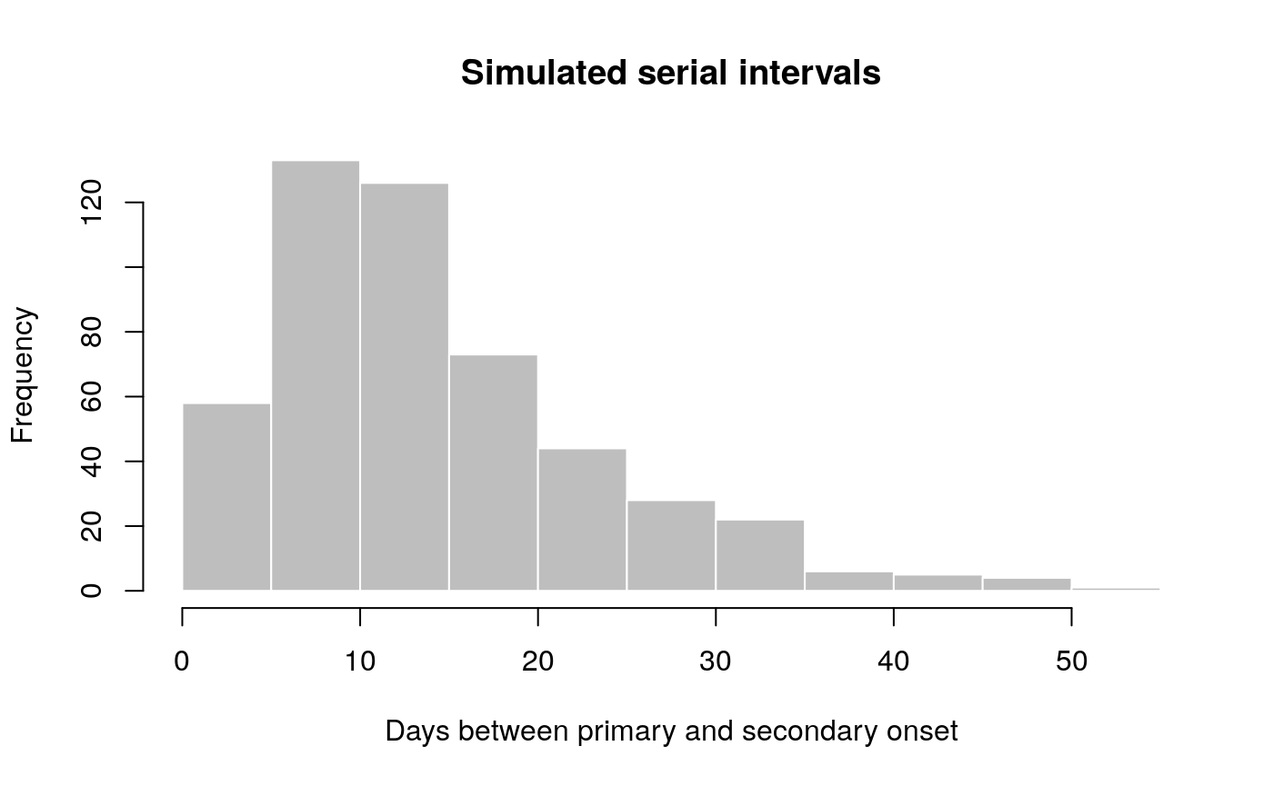

x contains simulated data, for illustrative purpose. In practice, one would use real data from an ongoing outbreaks. Now we use fit_disc_gamma to estimate the parameters of a dicretised Gamma distribution from the data:

si_fit <- fit_disc_gamma(x)
si_fit

## $mu
## [1] 15.21914
## 
## $cv
## [1] 0.5851581
## 
## $sd
## [1] 8.905604
## 
## $ll
## [1] -1741.393
## 
## $converged
## [1] TRUE
## 
## $distribution
## A discrete distribution
##   name: gamma
##   parameters:
##     shape: 2.92047557759351
##     scale: 5.21118646429829

Converting a growth rate (r) to a reproduction number (R0)

The package incidence can fit a log-linear model to incidence curves (function fit), which produces a growth rate (r). This growth rate can in turn be translated into a basic reproduction number (R0) using r2R0. We illustrate this using simulated Ebola data from the outbreaks package, and using the serial interval from the previous example:

library(outbreaks)
library(incidence)

i <- incidence(ebola_sim$linelist$date_of_onset)
i

## <incidence object>
## [5888 cases from days 2014-04-07 to 2015-04-30]
## 
## $counts: matrix with 389 rows and 1 columns
## $n: 5888 cases in total
## $dates: 389 dates marking the left-side of bins
## $interval: 1 day
## $timespan: 389 days
## $cumulative: FALSE

f <- fit(i[1:150]) # fit on first 150 days

## Warning in fit(i[1:150]): 22 dates with incidence of 0 ignored for fitting

plot(i[1:200], fit = f, color = "#9fc2fc")

## Registered S3 methods overwritten by 'ggplot2':
##   method         from 
##   [.quosures     rlang
##   c.quosures     rlang
##   print.quosures rlang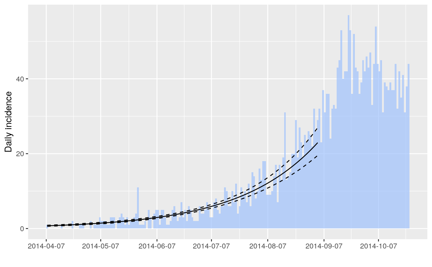

r2R0(f$info$r, si$d(1:100))

## [1] 1.348624

r2R0(f$info$r.conf, si$d(1:100))

##         2.5 %   97.5 %
## [1,] 1.314055 1.383674

In addition, we can also use the function lm2R0_sample to generate samples of R0 values compatible with a model fit:

R0_val <- lm2R0_sample(f$model, si$d(1:100), n = 100)
head(R0_val)

## [1] 1.350970 1.347374 1.350076 1.358523 1.341549 1.341634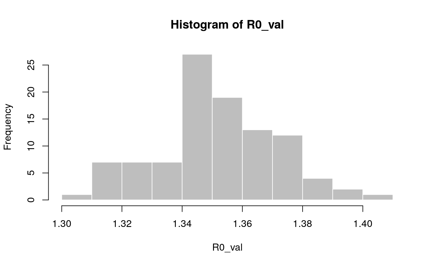

hist(R0_val, col = "grey", border = "white")

Standardising labels

If you want to use labels that will work across different computers, independent of local encoding and operating systems, clean_labels will make your life easier. The function transforms character strings by replacing diacritic symbols with their closest alphanumeric matches, setting all characters to lower case, and replacing various separators with a single, consistent one.

For instance:

x <- " Thîs- is A   wêïrD LäBeL .."
x

## [1] " Thîs- is A   wêïrD LäBeL .."

clean_labels(x)

## [1] "this_is_a_weird_label"

variables <- c("Date.of.ONSET ",
               "/  date of hôspitalisation  /",
               "-DäTÈ--OF___DîSCHARGE-",
               "GEndèr/",
               "  Location. ")
variables

## [1] "Date.of.ONSET "                "/  date of hôspitalisation  /"
## [3] "-DäTÈ--OF___DîSCHARGE-"        "GEndèr/"                      
## [5] "  Location. "

clean_labels(variables)

## [1] "date_of_onset"           "date_of_hospitalisation"
## [3] "date_of_discharge"       "gender"                 
## [5] "location"

Anonymising data

hash_names can be used to generate hashed labels from linelist data. Based on pre-defined fields, it will generate anonymous labels. This system has the following desirable features:

given the same input, the output will always be the same, so this encoding system generates labels which can be used by different people and organisations
given different inputs, the output will always be different; even minor differences in input will result in entirely different outputs
given an output, it is very hard to infer the input (it requires hacking skills); if security is challenged, the hashing algorithm can be ‘salted’ to strengthen security

first_name <- c("Jane", "Joe", "Raoul", "Raoul")
last_name <- c("Doe", "Smith", "Dupont", "Dupond")
age <- c(25, 69, 36, 36)

## detailed output by default
hash_names(first_name, last_name, age)

##             label hash_short
## 1     jane_doe_25     6485f2
## 2    joe_smith_69     ea1ccc
## 3 raoul_dupont_36     f60676
## 4 raoul_dupond_36     cd7104
##                                                               hash
## 1 6485f29654c5a9d55625cd6efeb96d569917e1c272790959ad3fa132c6d51648
## 2 ea1cccce320aa45a0d694ea12c30ff6b4b52c67f69d58b23dad5441ea17c5807
## 3 f60676d1c11ae5badc0e5ec4dfde06eaba817a78f3d54eb327a25df485ec1efd
## 4 cd7104e7e7009bfd988d5a4b46a930424908736065573e51a85d16575ed7c2a5

## short labels for practical use
hash_names(first_name, last_name, age,
           size = 8, full = FALSE)

## [1] "6485f296" "ea1cccce" "f60676d1" "cd7104e7"

Estimate incubation periods

The function empirical_incubation_dist() computes the discrete probability distribution by giving equal weight to each patient. Thus, in the case of N patients, the n possible exposure dates of a given patient get the overall weight 1/(n*N). The function returns a data frame with column incubation_period containing the different incubation periods with a time step of one day and their relative_frequency.

Load environment:

library(magrittr)
library(linelist)
library(epitrix)
library(distcrete)
library(ggplot2)

Make a linelist object containing toy data with several possible exposure dates for each case:

ll <- messy_data() %>% clean_data()

x <- 0:15
y <- distcrete("gamma", 1, shape = 12, rate = 3, w = 0)$d(x)
mkexposures <- function(i) i - sample(x, size = sample.int(5, size = 1), replace = FALSE, prob = y)
exposures <- sapply(ll$date_of_onset, mkexposures)
ll$dates_exposure <- exposures

print(ll)

##        id date_of_onset  discharge gender epi_case_definition messy_dates
## 1  zhugcj    2018-01-08 2018-01-18   male          not_a_case  1989-12-24
## 2  aeedki    2018-01-10 2018-01-20 female           suspected  2018-10-17
## 3  bjbblf    2018-01-07 2018-01-17 female          not_a_case  1989-12-24
## 4  nzigse    2018-01-11 2018-01-21   male           confirmed  2018-10-17
## 5  qivlvy    2018-01-09 2018-01-19   male            probable  2018-10-19
## 6  mlchbw    2018-01-06 2018-01-16 female           suspected  2001-12-01
## 7  zvipzg    2018-01-10 2018-01-20 female           suspected  2001-12-01
## 8  ewggll    2018-01-07 2018-01-17 female            probable  2018-10-19
## 9  zbttys    2018-01-07 2018-01-17 female          not_a_case  2018-10-19
## 10 ithycv    2018-01-09 2018-01-19 female            probable  2018-10-19
## 11 uupgyj    2018-01-06 2018-01-16 female            probable  1989-12-24
## 12 szcymp    2018-01-09 2018-01-19   male           suspected  2001-12-01
## 13 snsjbp    2018-01-04 2018-01-14   male           suspected        <NA>
## 14 ksxcgv    2018-01-09 2018-01-19 female          not_a_case  2018-10-19
## 15 wxlhwm    2018-01-06 2018-01-16   male           confirmed  2001-12-01
## 16 turjbi    2018-01-04 2018-01-14 female          not_a_case        <NA>
## 17 sljxly    2018-01-04 2018-01-14 female          not_a_case        <NA>
## 18 wfhwmk    2018-01-06 2018-01-16 female            probable  2018-10-17
## 19 mbhlsv    2018-01-04 2018-01-14 female           suspected  2018-10-19
## 20 wtcduu    2018-01-10 2018-01-20 female           suspected        <NA>
##          lat      lon                    dates_exposure
## 1  10.416562 48.68798               17538, 17533, 17537
## 2  14.819341 48.59420                             17538
## 3  10.784489 47.72968                             17534
## 4  12.231752 49.55408        17540, 17537, 17539, 17538
## 5  13.165470 47.48926                      17536, 17538
## 6  12.032235 47.70816                      17532, 17534
## 7   8.830518 49.10144        17539, 17538, 17537, 17536
## 8  15.335174 48.45867 17534, 17533, 17535, 17536, 17537
## 9  12.846348 48.85191        17534, 17532, 17531, 17535
## 10 14.060843 49.46620 17535, 17537, 17536, 17538, 17534
## 11 13.009818 48.24386                             17535
## 12 11.939537 48.64942                             17537
## 13 16.029733 47.35888               17531, 17532, 17530
## 14 14.630919 48.46446                      17537, 17536
## 15  9.986956 47.69080 17532, 17535, 17534, 17533, 17536
## 16 10.685640 49.27602                             17531
## 17 15.603110 47.95239               17532, 17531, 17529
## 18 11.188718 48.03010                      17531, 17532
## 19 13.031127 47.99642        17531, 17530, 17533, 17532
## 20 10.143990 45.96543 17538, 17537, 17539, 17540, 17536

Empirical distribution:

incubation_period_dist <- empirical_incubation_dist(ll, date_of_onset, dates_exposure)
print(incubation_period_dist)

## # A tibble: 8 x 2
##   incubation_period relative_frequency
##               <dbl>              <dbl>
## 1                 0             0     
## 2                 1             0.0467
## 3                 2             0.169 
## 4                 3             0.273 
## 5                 4             0.273 
## 6                 5             0.144 
## 7                 6             0.0808
## 8                 7             0.0125

ggplot(incubation_period_dist, aes(incubation_period, relative_frequency)) +
  geom_col()

Fit discrete gamma:

fit <- fit_gamma_incubation_dist(ll, date_of_onset, dates_exposure)
print(fit)

## $mu
## [1] 4.068634
## 
## $cv
## [1] 0.3322478
## 
## $sd
## [1] 1.351795
## 
## $ll
## [1] -1714.162
## 
## $converged
## [1] TRUE
## 
## $distribution
## A discrete distribution
##   name: gamma
##   parameters:
##     shape: 9.05890591579835
##     scale: 0.449130877853043

x = c(0:10)
y = fit$distribution$d(x)
ggplot(data.frame(x = x, y = y), aes(x, y)) +
  geom_col(data = incubation_period_dist, aes(incubation_period, relative_frequency)) +
  geom_point(stat="identity", col = "red", size = 3) +
  geom_line(stat="identity", col = "red")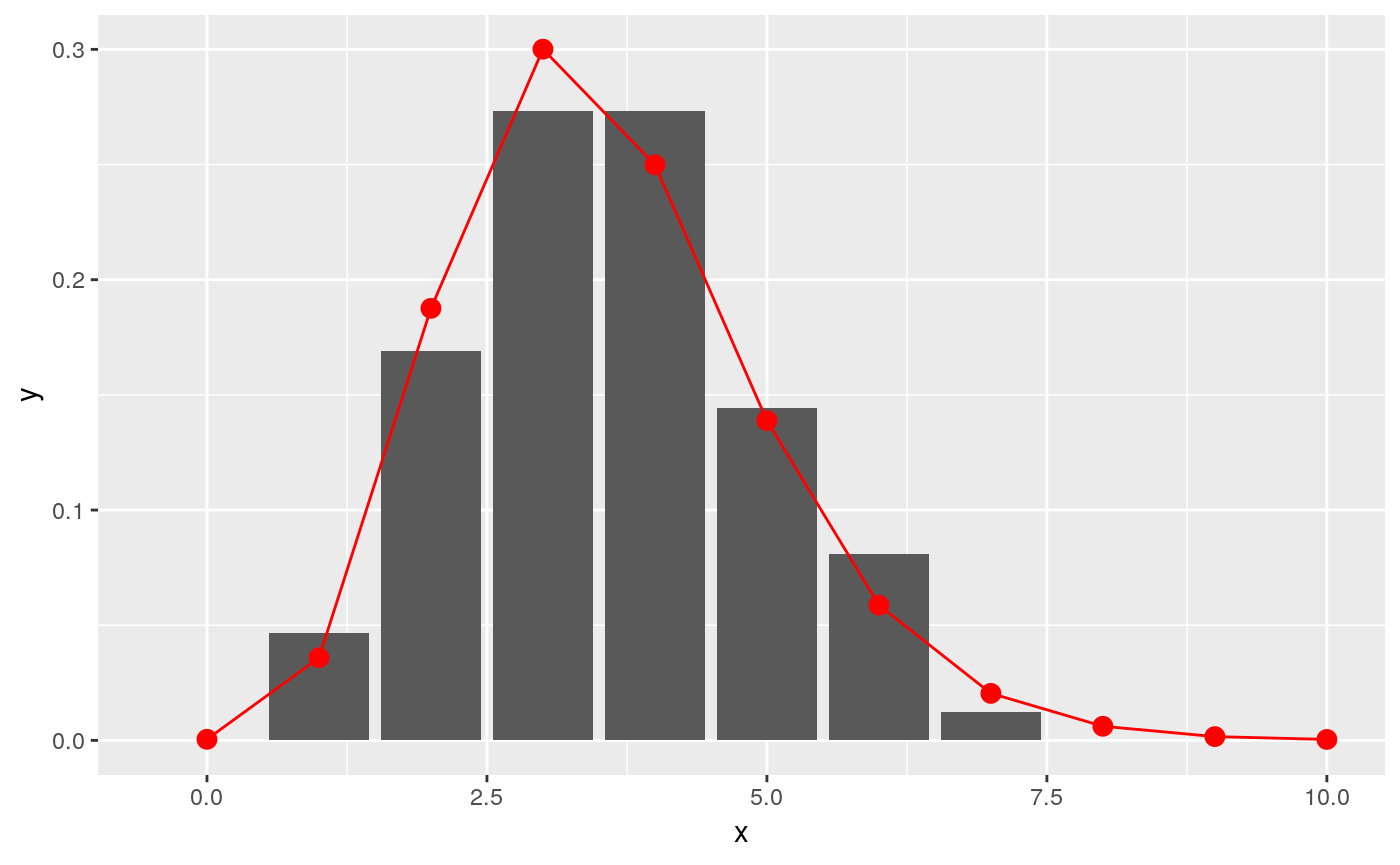

Note that if the possible exposure dates are consecutive for all patients then empirical_incubation_dist() and fit_gamma_incubation_dist() can take date ranges as inputs instead of lists of individual exposure dates (see help for details).

Vignettes

The overview vignette essentially replicates the content of this README. To request or contribute other vignettes, see the section “getting help, contributing”.

The estimate incubation vignette contains worked examples for the emperical_incubation_dist() fit_gamma_incubation_dist().